
Chapter Twenty One
Design II
- Introduction
- Construction Engineering: Concrete Mix and Formwork
- Environmental Engineering: Primary Treatment of Wastewater
- Geotechnical Engineering: Floodwalls
- Structural Engineering: Design of Structural Members
- Transportation Engineering: Horizontal Curves
- Outro
Learning Objectives
After reading this chapter, you should be able to:
- Design basic wood formwork for a concrete wall.
- Determine the dimensions of a primary clarifier for wastewater treatment.
- Explain the design principles for floodwalls.
- Design a beam to not exceed allowable stresses.
- Design horizontal curves of a roadway.
Introduction
In Chapter 10, we presented the design process and provided examples of how it is used in the subdisciplines of civil and environmental engineering. In the intervening chapters, we have presented many aspects such as economic, social, and sustainability considerations that are necessary in “real-world” design. In this chapter, we provide you with five design applications that take into account the additional considerations we have presented in Chapters 11 through 19.

Construction Engineering: Concrete Mix and Formwork
Concrete is often incorrectly referred to as “cement.” Cement is the binding agent in concrete, and is made by heating limestone and other materials at very high temperatures in a cement kiln. Concrete is a mixture of cement, water, and aggregate (sand and gravel, Figure 21.1). Concrete is typically about 10 to 15 percent cement, 60 to 75 percent aggregate, and 15 to 20 percent water on a volume basis. Important characteristics of concrete include its workability when wet, its final strength, and its durability after curing. Ready-mix concrete is concrete that is mixed to project specifications at a batch plant, either on-site or at a remote location.
Concrete may be enhanced by adding chemical or mineral admixtures. Admixtures can be used to:
- accelerate, or in some cases, retard curing times
- increase workability, durability, or strength
- add color for aesthetics
- inhibit corrosion of rebar
Waste products such as coal fly ash (fine particulates removed by air pollution control devices from coal-fired power plants) and ground blast furnace slag (from steel production) may be recycled into concrete as substitutes for a substantial fraction of the cement.
The amount of water in a concrete mix is critical to performance. A minimum amount of water must be added to initiate the chemical reactions that bind the cement to the aggregate. Additional water increases the workability of the concrete, so that it is not too “stiff.” However, as shown in Figure 21.2, the strength of concrete decreases as more water is added. Consequently, there is a tradeoff between strength and workability. Additionally, concrete strength increases with curing time (Figure 21.2).
Concrete is often poured, or placed, into forms (molds) to create columns, walls, and footings. Steel reinforcing bars (“rebars” or “rerods”) are often added to provide additional tensile strength. The forms are kept in place during initial curing.
Forms are typically removed as soon as possible once the concrete has cured to an adequate strength. The concrete will continue to cure and strengthen after the forms are removed. Temperature is very important to the rate of curing. At concrete temperatures below 70°F, curing slows (virtually stopping at 40°F). At higher temperatures, excessive evaporation of water from concrete can be problematic.
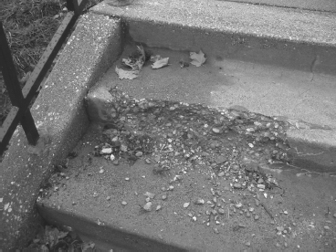
Figure 21.1 A Broken Concrete Step in Which Aggregate is Visible.
Source: M. Penn.
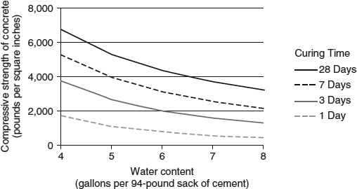
Figure 21.2 Ranges of Compressive Strength of Concrete as a Function of Water Content and Curing Time at 70°F.
Source: Adapted from Love, 1973.

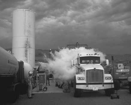
As concrete cures, chemical reactions increase the temperature. For the recently completed $240 million Colorado River Bridge bypassing the Hoover Dam, it was was determined that extreme desert heat (air temperatures exceeding 110°F) would result in curing temperatures that exceeded concrete design specifications. One approach to reducing curing temperatures is the circulation of water through pipes embedded in the concrete. However, this option was determined to be infeasible due to site-specific constraints. As a result, the seemingly extreme option of using liquid nitrogen to pre-cool the concrete before placement was used (Figure 21.3).
Figure 21.3 Liquid Nitrogen Being Injected into a Ready-Mix Truck to Cool Concrete Before Placement in the Construction of the Colorado River Bridge.
Source: Federal Highway Administration.
Concrete Canoes
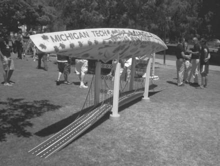
The American Society of Civil Engineers (ASCE) sponsors a concrete canoe competition annually. Students design lightweight concrete mixes, many of which are lighter than water, from which canoes are constructed (Figure 21.4). Although the races are the most exciting portion of the competition for the teams and spectators, 75 percent of the overall scoring is based on a design report, an oral presentation, aesthetics, and durability.
 ASCE National Concrete Canoe Competition Rules and Regulations
Figure 21.4 A Concrete Canoe on Display at the 2010 National Competition Hosted by the California Polytechnic State University-San Luis Obispo. This canoe placed third nationally in the Final Product category, and fourth overall. The display stand is a model of the Mackinac Bridge, the third longest suspension bridge in the world, which spans the Mackinac Strait between Lake Michigan and Lake Huron.
Source: Courtesy of Michigan Technological University, ASCE 2009-2010
Concrete Canoe Team.

Figure 21.5 Forms for a Concrete Wall
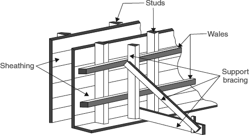
The design of formwork is necessary for efficient construction and to ensure that the final product meets design specifications for shape, surface finish, and strength. Examples of forms for walls and columns are shown in Figure 21.5 and Figure 21.6 respectively. Formwork at a construction site is shown in Figure 21.7.
The design of formwork involves the temporary structural support for the sheathing that acts as the mold for concrete. The formwork must support the hydrostatic pressure of the freshly placed concrete, the weight of construction workers, the weight of equipment, and the impact of vibration if used to consolidate the concrete. Formwork may be of wood, aluminum, steel, fiberglass, or foam board.
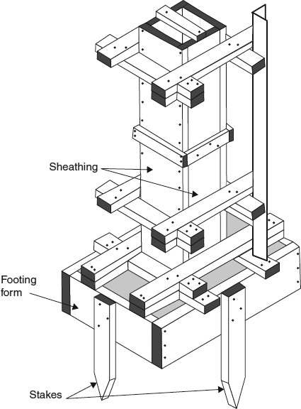
Figure 21.6 Forms for a Concrete Column and Footing.
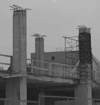
Figure 21.7 Formwork on Second-Story Columns (Right), and Cured Columns After Form Removal (Left, Background, and Below). Note the rebar projecting from the tops of the columns.
Source: M. Penn.
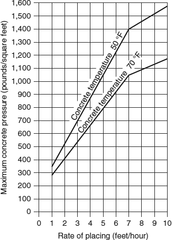
Figure 21.8 Concrete Pressure on Form Sheathing as a Function of Concrete Placement Depth Rate. Note that for a given depth, the hydrostatic pressure of freshly poured concrete is approximately 2.5 times greater than that of water since the unit weight of concrete is approximately 2.5 times greater than that of water (150 lbs/ft3 for concrete, 62 lbs/ft3 for water).
Source: Adapted from Love, 1973.
Simplified wood formwork design will be presented here for construction of a concrete wall. First, consider that the hydrostatic pressure of the placed concrete on the form sheathing is a function of both temperature and the rate (i.e., depth per time) of concrete placement in the form. This is demonstrated in Figure 21.8.
The rate of concrete placement is important because as concrete begins to cure, or “set,” the hydrostatic pressure decreases. When fully cured, concrete exerts no hydrostatic pressure on the forms. Consequently, higher placement rates will lead to a greater depth of liquid concrete, which will exert higher hydrostatic pressure as shown in Figure 21.8. Figure 21.8 also demonstrates that, all other things being equal, higher temperatures decrease the maximum concrete pressure; this is due to the fact that higher temperatures lead to faster curing.
Higher pressures require stronger formwork to prevent deflection of the sheathing and potential seepage of wet concrete between sheathing panels, termed blowout. Thus, there is a tradeoff between rate of concrete placement and the cost and time of erection of the formwork. Construction engineers must balance this tradeoff to decide what is best for a given project depending on budgets and timelines.
Once the desired placement rate and resultant concrete pressure is determined, the stud spacing to support the sheathing can be determined based on the type of sheathing (Figure 21.9). Note that as the sheathing thickness increases, so does the stud spacing. Thicker sheathing provides additional resistance to the concrete pressure, requiring less stud support. For example, at a concrete pressure of 800 pounds per square feet, 1-inch plywood sheathing requires 14-inch stud spacing compared to 8-inch spacing for 1/2-inch plywood sheathing.
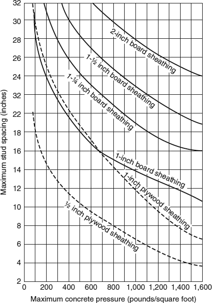
Figure 21.9 Maximum Stud Spacing as a Function of Concrete Pressure.
Source: Adapted from Love, 1973.
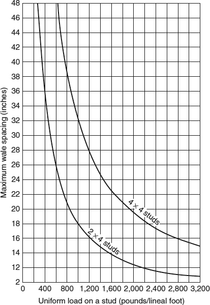
Figure 21.10 Wale Spacing as a Function of Stud Size and Stud Loading.
Source: Adapted from Love, 1973.
The stud loading (pounds/lineal foot) is equal to the product of concrete pressure pounds/square feet and stud spacing (feet). The vertical studs are cross-supported, horizontally, by wales (refer to Figure 21.5). The wale spacing is determined from Figure 21.10 based on the calculated stud loading and the stud dimensions. Note that wale spacing increases with stud size, as larger studs require less support. For example, a load of 1,000 pounds/lineal foot requires 18-inch spacing for 2-inch × 4-inch studs as compared to 32-inch spacing for 4-inch × 4-inch studs. The construction engineer again is faced with a tradeoff, this time between stud size (and cost) and the number of wales needed for support.
numerical example 21.1 Form Design
Determine the 2-inch × 4-inch stud and wale spacing to support 1-inch plywood forms for a concrete wall that is to be placed at a rate of 5 feet per hour with a concrete temperature of 70°F.
According to Figure 21.8, the concrete pressure on the forms will be 800 pounds/square feet.
Next, the stud spacing required is found to be approximately 14.2 inches by using Figure 21.9. This spacing is rounded down to 14 inches for ease of measurement in the field. Note that this also makes the design slightly conservative; by rounding down, rather than up, we are ensuring that the stud spacing is more than sufficient to support the concrete pressure.
The stud loading is determined by:
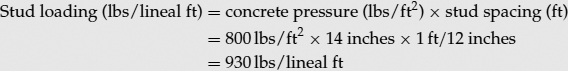
Using this stud loading and Figure 21.10, the wale spacing for 2-inch × 4-inch studs is found to be approximately 18.5 inches. Again, this is rounded down to 18 inches to incorporate a modest safety factor.
Because of cost savings, modular form systems made of aluminum or steel (Figure 21.11) are replacing wood forms in practice. Modular forms last longer than wood, and require less time to install. The modular sections are pinned or clipped together, and wood or aluminum wales are fastened horizontally to provide deflection support as required.
Variations of Formwork
Not all formwork is temporary (i.e., removed after curing). Permanent insulated concrete forms are becoming increasingly popular as energy prices rise.
Not all formwork is used to cast concrete in-place. Precast concrete panels, or tilt-up concrete walls are formed and cured in a controlled environment either onsite, or offsite and transported to a construction site for placement.
Information on Insulated Concrete Forms
Time-Lapse Video of Insulated Concrete Form Installation
Tilt-Up Concrete Panels Product Information
There are many types of concrete that have particular advantages with regard to constructability, design strength, durability, and aesthetics. You will learn about these, as well as how to design concrete mixes (relative amounts of water, cement, and aggregate, as well as the size of aggregate), in future civil engineering courses.
![]() Remember that full-sized versions of textbook photos can be viewed in color at www.wiley.com/college/penn.
Remember that full-sized versions of textbook photos can be viewed in color at www.wiley.com/college/penn.
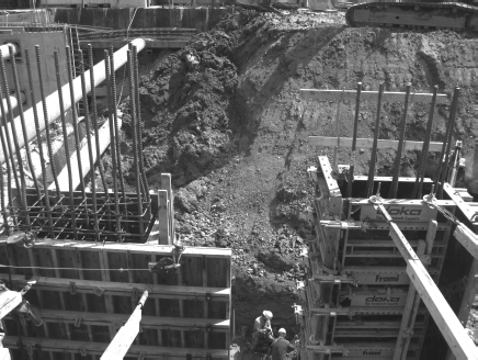
Figure 21.11 Wooden Forms (Left) and Modular Forms (Right) for Reinforced Concrete Foundation for a High-Rise Building in Downtown Chicago.
Source: P. Parker.
Environmental Engineering: Primary Treatment of Wastewater
Wastewater treatment processes were introduced in Chapter 5. Here we will provide you with the fundamental design concepts of primary treatment. Primary treatment follows preliminary treatment that removes grit and debris. The objective of primary treatment is to remove floatable solids (fats, oils, and greases) and readily settling solids (organic and inorganic particles). The settling of particles leads to “clearer” water and thus settling tanks are termed clarifiers. Stokes' Law (Equation 21.1) is often used to estimate settling velocities.
where
Vs = settling velocity (m/s)
g = gravitational constant (9.8 m/s2)
d = particle diameter (m)
ρp = particle density (kg/m3)
ρw = wastewater density, temperature dependent (kg/m3)
μ = viscosity1 of wastewater, temperature dependent (kg/ms)
A pair of primary clarifiers are shown in Figure 21.12. Floatable solids are skimmed from the water surface of the tank and collected in a sump before being pumped to a digester for further treatment. After settling to the tank bottom, settled solids are scraped to an accumulation hopper (Figure 21.13) and then pumped to a digester.
In reality, wastewater contains particles of all shapes, sizes, and densities, thus limiting the use of Stokes' Law. It is common in engineering to develop empirical relationships based on collected data for use as the basis for design. One such relationship will be used here.
Figure 21.12 Twin (Parallel) Primary Clarifiers in Platteville, Wisconsin. Wastewater enters the tanks in background and exits in foreground. 1: Accumulated floatables on water surface. 2: Skimmer blades push floatables to the accumulation area for removal. The twin tanks provide redundancy, to allow partial treatment in one tank while the other is being repaired or undergoing maintenance. Under normal conditions, both clarifiers are used in parallel, each treating one-half of the influent.
Source: M. Penn.
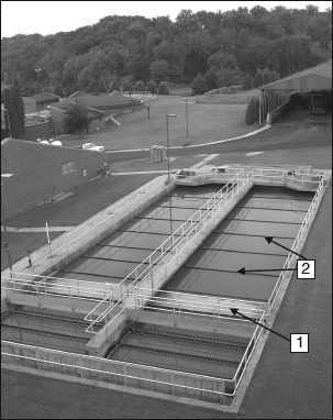


Figure 21.13 Side View of a Simplified Primary Clarifier.
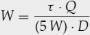
First, consider that for primary clarifiers, the percentage of particles (also termed suspended solids, SS) removed increases as a function of the time that the wastewater is in the clarifier (detention time, τ).
where
τ = detention time (hr)
V = volume of tank (m3)
Q = flowrate of wastewater through the tank (m3/hr)
The relationship between detention time and removal efficiency is shown in Figure 21.14 for both SS (which includes inorganic and organic solids) and BOD, or biochemical oxygen demand. BOD is the target contaminant for removal in the subsequent secondary treatment step.
BOD, or biochemical oxygen demand, is a measure of the degradable organic content of the wastewater.
Note from Figure 21.14 that the removal efficiency dramatically increases with detention times up to about 2 hours, and begins to plateau after approximately 4 hours. Particles that are not removed are very small and settle very slowly. In Stokes' Law, the settling velocity is a function of the diameter squared; thus, a 0.01-mm diameter particle settles 100 times slower than a 0.1mm particle of the same density. The typical design detention time is 2 hours for primary clarifiers. Longer times require larger and more expensive tanks, which provide only a minimal increase in treatment efficiency, and thus are not cost-effective.
Using a specified detention time and a known design flowrate of wastewater, the required volume of the tank can be determined by solving Equation 21.2 for volume. If rectangular in shape, the length (L), width (W), and depth (D) must be determined based on the volume. Most states have design codes that stipulate the minimum depth of primary tanks. Typical depths of primary tanks are 4 meters. What remains to be determined is the length and width of the tank. A long and “skinny” tank is impractical from a construction excavation standpoint. A short and “wide” tank is subject to inefficient treatment as the wastewater may “short circuit” the tank (exiting before its designed detention time). Typical length-to-width ratios are 5:1.
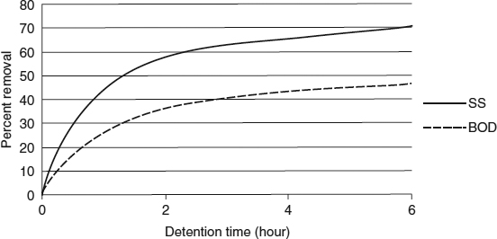
Figure 21.14 Removal of SS and BOD in Primary Clarifiers as a Function of Detention Time.
Source: Adapted from Steel & McGhee, 1979.
numerical example 21.2 Preliminary Sizing of Primary Clarifier
For a wastewater flowrate of 150 cubic meters/hour and a specified detention time of 2 hours, calculate the dimensions of a primary clarifier. The tank depth is 4 meters and the length-to-width ratio is 5.
solution
In order to determine the dimensions of primary clarifiers for site layout and structural design purposes, we can solve Equation 21.2 for tank volume:
Tank volume = τ.Q
The volume of the tank is the product of the tank's length, width, and depth, and his relationship can be substituted into the previous equation.
τ.Q = L . W.D
Thus, we can rearrange for tank width:
![]()
Substituting the given length-to-width ratio yields the following:
Solving for W yields the following:
![]()
For a wastewater flowrate Q of 150 cubic meters/hour and a specified detention time τ of 2.0 hours, the tank dimensions would be (L × W × D): 19 meters by 3.9 meters by 4.0 meters. If two parallel redundant tanks were to be used, the surface area, SA, of each tank would be halved:
SA = L.W = 19m × 3.9m/2 = 37m2.
The L:W ratio would remain 5; thus the dimensions can be determined:
L.W =5W2 = 37m2.
The width of each tank would be 2.7 meters and the length would be 13.6 meters.
Additional design requirements for primary clarifiers include:
- Selection of skimmer/scraper to remove settled solids and floatables (these are designed by manufacturers and selected or specified by environmental engineers.
- Design of sumps for collected solids (sludge) at the bottom of the tank and floatables.
- Hydraulic design of influent and effluent flow control structures to ensure mixing at the entrance and to minimize resuspension of settled solids at the entrance and exit by reducing wastewater velocities.
- Hydraulic design of pumps and piping to transport removed floatables and settled solids to the digester.
- Structural design of the reinforced concrete for the tank walls and base.
- Selection of tank covers (in some instances) to control odors.
Geotechnical Engineering: Floodwalls
Cantilevered floodwalls are often referred to as “T-walls” because the cross-section has the shape of an inverted “T” (Figure 21.15). T-walls are designed to prevent three common types of floodwall failure: sliding, overturning, and exceeding soil-bearing capacity. Sliding occurs when lateral forces on the water side of the floodwall exceed resisting forces of the supporting soil (Figure 21.16). Overturning occurs when a wall rotates along the base of the toe (Figure 21.17). Bearing capacity failure occurs when the pressure on the soil at the base of the wall exceeds the bearing capacity of the soil (Figure 21.18).
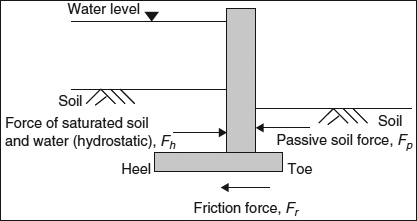
Figure 21.15 A Cantilevered Floodwall, or T-Wall. Horizontal forces acting on the wall are shown.
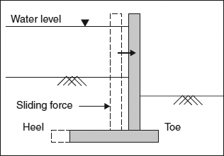
Figure 21.16 Failure of a T-Wall by Sliding.
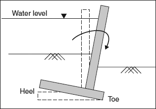
Figure 21.17 Failure of a T-Wall by Overturning. Note the rotation occurs at the toe.
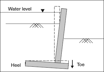
Figure 21.18 Failure of a T-Wall Due to Excessive Soil Pressure and Settlement. Note that the base has settled, primarily at the toe.
Figure 21.19 Failure of an I-Wall Due to Scour of Supporting Soil Due to Overtopping of the Floodwall. The base of a T-wall (not shown) provides additional protection from scour due to overtopping water.
Source: Adapted from ASCE, 2007.
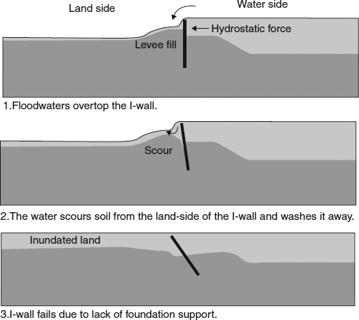
Preventing bearing capacity (settlement) failure in foundations is the purpose of footings, which you learned to design in Chapter 10. T-walls also minimize the risk of failures from excessive scour of soil on the land side of the wall due to overtopping of the floodwall by high water (Figure 21.19), which occurred at some I-walls (a vertical wall without a horizontal base) during Hurricane Katrina. In this section, we will discuss floodwall design to prevent sliding failure.
In order to prevent sliding failure, the resistive lateral forces of the soil must be greater than the cumulative lateral sliding force, FH, of the water (hydrostatic) and of the saturated soil on the high water side of the wall (Figure 21.15). A factor of safety of 1.5 is typically used in designs, such that: Sum of resistive forces/Sum of sliding forces ≥ 1.5.
The resistive forces are the friction force, FR, at the base of the footing and the passive soil force, Fp, above the base of the toe (Figure 21.15). The passive soil force is a function of the soil depth above the base and the passive soil pressure coefficient, Kp, which is a measure of the lateral pressure that a soil type can withstand without movement. In simple terms, imagine the passive soil force as the force resisting the blade of a bulldozer. The bulldozer must overcome this force in order to move the soil. The greater the Kp of the soil, or the greater the soil depth on the blade, the more force required by the bulldozer.
The second lateral resisting force, the friction force, is the product of the soil coefficient of friction, Cf, and the net (downward) vertical force acting on the base. The friction force acts laterally along the base of the T-wall. In simple terms, again using the bulldozer example, the friction force is equal to the force required by a bulldozer to push (slide) an object along a soil surface. The net vertical force, and thus the friction force, increases as the base width, B, increases (increasing the weight of the concrete base) and as the height of soil above the heel or toe, Dh or Dt increases (increasing the weight of soil acting on the base).
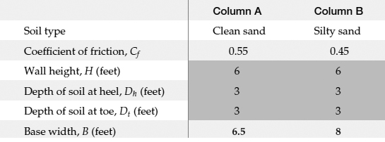
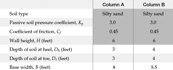
Design values for T-wall base widths are provided in Table 21.1 and Table 21.2 for two scenarios:
Table 21.1 Base Width Design for Scenario 21.1 Common parameters are shaded.
Source: Adapted from FEMA, 2001.
Scenario 21.1: Different soil types with all other parameters being equal (Table 21.1). The soil types are clean sand (without fines) and silty sand (with fines), each with different values of Kp and Cf.
Scenario 21.2: Different soil depths (over both toe and heel of the base) with all other parameters being equal (Table 21.2). The soil depths considered are 3 feet and 4 feet.
By comparing columns A and B in Table 21.1, we can see that for different soil types, the base width increases from 6.5 feet to 8 feet because the silty sand has a lower value of Kp and Cf than clean sand. By increasing the base width in silty sand, the net vertical force increases, which results in more weight of concrete in the base and more weight of soil above the enlarged base. This increased net vertical force counteracts the lower Cf, and increases the resistive friction force. In this case, changing the base width does not affect the passive soil force, because the depth of soil remains constant.
By comparing columns A and B in Table 21.2, we can see that when the soil depth increases from 3 feet to 4 feet over the base (for the same soil type), the base width decreases from 8 feet to 5.5 feet. The increased soil depth results in an increased net vertical force and thus an increased frictional resistive force for any given base width. Also, the passive soil force increases with soil depth for a constant value of Kp.
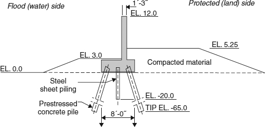
This simplified design approach does not incorporate all of the forces that may be acting on a floodwall. Actual design may require accounting for additional soil and hydrodynamic forces that you will learn about in a geotechnical engineering course (in which you will also gain the technical knowledge to design floodwalls in order to prevent overturning and pressure failures not covered in this section). For example, in “soft” soils with low bearing capacities, the foundation is extended to greater depths (Figure 21.20).
Table 21.2 Base Width Design for Scenario 21.2 Common parameters are shaded.
Source: Adapted from FEMA, 2001.
Figure 21.20 Extended Foundation of a T-Wall in Soft Soil. Typical elevations (abbreviated as “EL.” in diagram) and dimensions shown. Note concrete piles extend 65 feet below the base of the T-wall.
Source: USACOE.
Structural Engineering: Design of Structural Members
As we discussed in Chapter 20, a structure must be able to support ultimate loads without failing, and must also support service loads without deflecting or vibrating excessively. In this section, we will discuss the concept of designing a beam to accommodate an internal stress such that it will not fail when subjected to ultimate loads.
In structural engineering, stress is defined as a force per area. To understand the concept of stress, consider the cantilevered member of Figure 21.21. The beam is being subjected to an axial force and is in tension. This force is carried throughout the entire member. When analyzing the interior cross-section of the member as shown in Figure 21.22, this force F is distributed across the cross-sectional area A. The stress, a, may be defined with the variables of Figure 21.21 and Figure 21.22 using Equation 21.3.
where
F = force applied
A = cross-sectional area
b = structural member width
h = structural member height
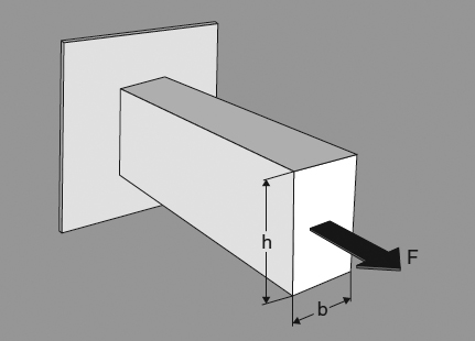
Figure 21.21 A Cantilevered Structural Member in Tension.
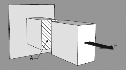
Figure 21.22 Internal Cross-Sectional Area (A, Hatched) of Structural Member Across Which the Tensile Force is Distributed.
For common SI units of newtons for force and m2 for cross-sectional area, stress has units of N/m2, which is equal to one pascal (Pa). The stresses involved in structural engineering are relatively large, and are often expressed as MPa (megapascals, or 106 Pa). For English units, common units are lb (force), in2 (area), and psi or pounds per square inch (stress).
You can readily imagine that the member in Figure 21.21 and Figure 21.22 could withstand a certain force before it failed (i.e., “broke”). Certain materials are “strong” in the sense that a large force per unit area is needed before they fail as compared to “weak” materials. Said another way, stronger materials can withstand larger stress.
The engineer designing a beam needs to ensure that it does not fail when subjected to ultimate loads. One method to do so is to calculate the stress carried by a beam and compare it to the beam's failure stress. For this textbook, we will term this method of analysis and design the maximum permissible stress method. While this exact method is not used by practicing engineers, it is based on the same concepts used in practice, and is simplified for use by first-and second-year students.
Failure stress is the stress that a structural member can carry before it fails.
The calculation of stress for a simply supported beam is somewhat more complex than for a cantilevered structural member under pure tension. For a simply supported beam loaded at its center, the maximum permissible stress carried by the beam is given by Equation 21.4, where the subscript “ss” refers to the simply supported beam. In future structural engineering courses, you will learn how to derive this equation and similar equations for other beam arrangements (e.g., cantilevered beam, simply supported beam carrying a distributed load).
where
L = beam length
F = magnitude of point load at center of simply supported beam
σss = maximum permissible stress.
To analyze a beam to determine whether it could carry its ultimate loads, Equation 21.4 would be solved for the maximum permissible stress, given F (value for the ultimate load) and the beam dimensions (width, height, and length). The maximum permissible stress would then be compared to the ultimate stresses corresponding to the material type using Table 21.3. Theoretically, if the stress calculated using Equation 21.4 is less than the stress in Table 21.3, then the beam will not fail. However, in reality, σss should be less than the ultimate stress in Table 21.3 by a considerable amount as determined by the factor of safety (FS), defined by Equation 21.5. A typical value for FS is 1.5; thus, the value of the maximum permissible stress calculated using Equation 21.4 should be at least 1.5 times less than the ultimate stress of the material.
Table 21.3 Ultimate Stresses for Various Materials
| Material | Failure Stress (psi) |
| Aluminum | 60,000 |
| Concrete | 500 |
| Pine wood | 6,000 |
| Stainless steel | 75,000 |
| Steel | 36,000 |
To design a beam, a similar process would be followed. The designer can manipulate several variables, including the beam material and cross-sectional dimensions. A factor of safety will likely be specified by industry design standards.
numerical example 21.3 Preliminary Sizing of a Beam
Consider a simply supported steel beam that needs to carry a load at its center of 2,000 pounds. The beam length is 15 feet (180 inches). If the beam height is to be twice its width and a factor of safety of 1.5 is to be used, determine the beam's height and width using the maximum permissible stress method.
solution
From Equation 21.5, σss can be calculated by knowing the factor of safety and the ultimate stress of steel, obtained from Table 21.3.
![]()
Thus, we must ensure that the beam cross-section is large enough that the stress developed is less than 24,000 psi. We can now use Equation 21.4 to calculate the dimensions that can effectively carry this stress. Given that the height is to be twice as large as the width, we can substitute into Equation 21.4 the expression h = 2b.
![]()
This equation can be solved for b, knowing values of σss, F, and L. L will be inserted using units of inches to keep units consistent.
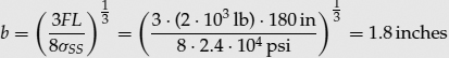
Given this value of b, we conclude that the height h is 3.6 inches.
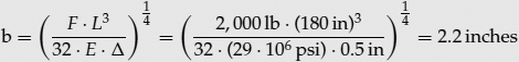
numerical example 21.4 Redesign of a Beam, Considering Beam Deflection
A beam of the dimensions calculated in Numerical Example 21.3 should structurally withstand the specified load. Reflecting on Chapter 20, perhaps you are asking, “I wonder if the beam will deflect too much?” Using the rule of thumb that the deflection should be less than 1/360 of the beam length (0.042 foot or 0.5 inch in this case), we can investigate whether this beam will deflect excessively.
solution
To calculate the deflection, we will use Equation 20.4 from Chapter 20. To keep units consistent, the beam length L will be inserted with units of inches.
![]()
We can conclude that although the beam will not break when a force of 2,000 lb is exerted, it will deflect too much. Consequently, the beam needs to be re-designed to ensure that deflection is within allowable limits. We will determine the necessary cross section dimensions by solving Equation 20.4 from Chapter 20 for b (knowing that h = 2 · b and Δ = 0.5 inches).
Given this value of b and the specified height-to-width ratio, the beam height, h, equals 4.4 inches. A beam with these dimensions will not deflect “too much.” Since these dimensions are larger than the original beam we designed, we can be sure that the stress in the beam will be much lower than the ultimate stress. This can be confirmed by inserting the dimensions into Equation 21.4; the result demonstrates that the ultimate stress in the simply supported beam will be less than the previously determined design criteria for stress of 24,000 psi.
![]()
This design results in a FS value of 1.9 (36,000 psi/19,000psi).
Transportation Engineering: Horizontal Curves
In plan view, roads are composed of straight sections, termed tangents, and horizontal curves. A horizontal curve provides a transition between two tangents and facilitates the movement of traffic between the two tangents. The tangents meet at an imaginary point of intersection (POI) as shown in Figure 21.23.
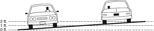
The radius of the horizontal curve and the amount of superelevation dictate the speed at which a vehicle can move through a horizontal curve. The cross slope of superelevation is often expressed as a percent, where a superelevation of 5 percent would describe a road cross-section that has a slope of 0.05 feet of rise (vertical) per 1 foot of run (horizontal). This is similar to our previous discussion on road crowns in Chapter 4, Transportation Infrastructure, in which the normal cross section of a road has a cross slope of 2 percent downward from the centerline crest. Figure 21.24 provides a scaled drawing of a 40-foot wide roadway superelevated at 5 percent.
Superelevation refers to the extent that a curve is banked or tilted in cross-section. It is also known as camber or cross slope.
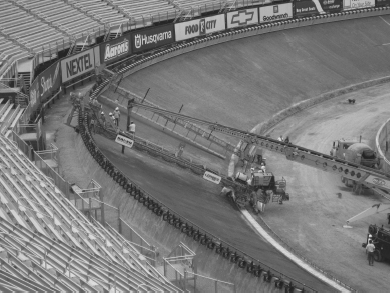
Intuitively, most people understand that as the radius of a curve increases, a vehicle can move through that curve more rapidly. Tight curves (i.e., curves with small radii) require low speeds while large radius curves allow a higher travel speed. In addition, as the rate of superelevation increases, the rate at which vehicles can safely move through the curve increases. This is the reason that automobile race tracks are superelevated at very high slopes; for example, the Bristol Motor Speedway (Figure 21.25) has a superelevation of 10 percent, which corresponds to 36° and is the steepest superelevation of any NASCAR track. To put this in perspective, 36° is the approximate slope of an Olympic ski jump or a “black diamond” downhill ski run.
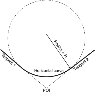
Figure 21.23 A Horizontal Curve Between Two Tangents and the Point of Intersection (POI) of the Tangents.
Figure 21.24 Roadway with Superelevation of Five Percent.

Equation 21.6 is a governing equation for the design or horizontal curves, and agrees with intuition as it takes into account the rate of superelevation and the curve radius. In addition, the friction between the vehicle's tires and the roadway surface will affect the design radius. Note that Equation 21.6 is a non-homogeneous equation; you must use the units specified in order for the radius to be calculated in units of feet.
where
R = radius of curve (ft)
v = velocity of vehicle in curve (mi/hr)
e = rate of roadway superelevation (ft/ft)
f = side friction factor, expressed as a decimal
Figure 21.25 The Resurfacing of Bristol Motor Speedway. This photograph illustrates the superelevation of a NASCAR racetrack.
Source: Courtesy of Baker Concrete Construction.
![]() Remember that full-sized versions of textbook photos can be viewed in color at www.wiley.com/college/penn.
Remember that full-sized versions of textbook photos can be viewed in color at www.wiley.com/college/penn.
numerical example 21.5 Horizontal Curve Design
A rural road has been designated for resurfacing and realignment. Currently, it has a design speed of 55 mph, but a horizontal curve between two perpendicular tangents is only designed for 25mph.
- Calculate the radius of the existing curve if the curve is not superelevated and the side friction factor is 0.1.
- When realigning the road, engineers wish to use a design speed of 45mph for the curve. How might they achieve this?
We address this problem by using Equation 21.6, given that e = 0 and f = 0.1. These values can now be substituted into Equation 21.6.
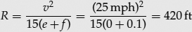
- We have two variables to manipulate in Equation 21.6, e and R, and thus there are an infinite number of solutions. For example, if the curve is superelevated to 4 percent (e = 0.04), using Equation 21.6 with a velocity of 45 mph and side friction factor of 0.1 yields a radius of 960 feet. Alternatively, a superelevation rate of 6 percent decreases the radius to 840 feet. Choosing the appropriate superelevation rate and radius would be accomplished by referring to appropriate codes and standards, as well as considering land use issues and construction costs.
As we have emphasized in this textbook, engineering consists of much more than inserting values into equations and solving those equations. This is certainly true in the case of horizontal curve design. For example, as the designed radius of a curve increases, the amount of land required will also increase. As a result, more property will be affected; this affected property might be very expensive to purchase, or may include wetlands or other environmentally sensitive areas. If the land is privately owned, the potential for conflict with landowners will increase. Also, safety is paramount in the design of horizontal curves. When the radius requires a lower speed limit than that of the incoming tangent, the potential for accidents increases. Small-radius curves, by making vehicles deccelerate and then accelerate, are less fuel efficient than large-radius curves. Moreover, designers must take into account transitions between crowned cross-sections of tangents and superelevated cross-section of curves.
Flash Animation of Roadway Transitions
“Dead Man's Curve”
One of the few 90-degree curves in the Interstate Highway System exists along I-90 in Cleveland, Ohio (Figure 21.26). It was first opened to traffic in 1962 with a 50-mph speed limit. Many accidents, including truck rollovers, occurred. In 1965, the posted speed limit was lowered to 35 mph, but the accidents continued. In 1969, the curve was superelevated and the median guardrail was replaced with a concrete barrier. Recently, larger signs, better night-time lighting, and flashing warning lights have been added.
Mahmoud Al-Lozi, a highway system planner for the Northeast Ohio Areawide Coordinating Agency, commented on why the accident rate remains high, despite all of the efforts to increase driver safety, “They get used to traveling curves posted at 45 mph at 55 mph with no problems, so when they encounter a bad one, they're not ready for it. Dead Man's Curve is one of those where they say 35 mph and they mean 35 mph” (Sweeney, 2001).

Figure 21.26 A Sign Alerting Drivers to “Dead Man's Curve” on I-90 in Cleveland, Ohio. Note that this is not an off-ramp.
Source: P. Parker.

Figure 21.27 Existing and Proposed Alignment.
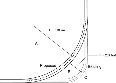
We can see the effect of curve radius on consumption of land by considering a hypothetical case.Figure 21.27 illustrates an existing and proposed alignment. The proposed alignment is presented as dark lines and the existing alignment as light lines. Offsets have been drawn 15 feet to the side of each centerline to represent the edge of pavement. For each case, the dashed line is the circular arc segment that comprises the horizontal curve.
The length of the proposed redesigned horizontal curve is 960 feet, which multiplied by a pavement width of 30 feet, yields a road area of 29,000 square feet, or 0.67 acres. Additional land will need to be purchased beyond the edge of pavement for the right-of-way. If the right-of-way width is 40 feet (20 feet from the centerline), the total land area to be acquired is 0.88 acres. Depending on property values in the area, the cost of this land may amount to a significant fraction of the total project cost. In addition, the design engineers must address this question: what should be done with the land between the proposed and existing alignment (denoted with a ‘B’ in Figure 21.27)? This land has an area of 0.93 acres, and most likely belonged to property owner A before construction began, but may have little or no value to the owner as it is no longer contiguous with his or her property. Moreover, property owner C may have no use for the land either. In such a case, the road owner (e.g., the county, state, or township) may need to purchase that land also from property owner A and be responsible for maintaining that land in the future.
The values reported in the previous paragraph were obtained from the computer aided drafting (CAD) program with which Figure 21.27 was drawn. You can easily replicate this work in any CAD program; alternatively, answers with satisfactory precision can be obtained by use of a compass, protractor, and engineering scale.
Outro
In future engineering courses, you will be able to analyze and design much more complicated infrastructure components than we have presented in this book. We hope that in your future courses, where the tendency may be to focus on technical topics, that you continue to view infrastructure components and sectors in light of the many non-technical considerations that we have presented in this textbook.
chapter Twenty One Homework Problems
- 21.1 Reconsider Numerical Example 21.5. What is the radius of the redesigned curve if there is no superelevation? How does your answer compare to the answers provided in the example?
- 21.2 Reconsider Numerical Example 21.5. One way to increase the allowable traffic speed around the curve is to increase the side friction factor f. If the pavement is constructed of concrete, it can be diamond-ground, effectively increasing f from 0.1 to 0.18. Alternatively, a type of asphalt overlay termed “open-graded friction course” can increase f from 0.1 to 0.15.
- For the existing curve (i.e. radius is 420 feet and no superelevation), how much will these two rehabilitation techniques increase the design speed of the existing curve?
- The asphalt overlay can be applied in such a way to increase superelevation. How much will increasing e to 0.4 and 0.6 increase the design speed for the existing curve?
- 21.3 Use a spreadsheet to create a graph of minimum curve radius as a function of vehicle speed, given that e = 0.0 and f = 0.15. Show vehicle speed on the x-axis, varying from 0 to 60 mph.
- 21.4 Two horizontal tangents meet at a 90° angle. For a 55 mph design speed, design two “safe” curves, specifying values of e, f, and R for each of your designs. Also, use a CAD program or a careful hand drawing to estimate the horizontal curve length of each of your designs.
- 21.5 A community of 510,000 people generates wastewater at a rate of 105 gallons/capita/day. The community is growing at a rate of 0.50 percent per year. When designing a new WWTF, design flows are typically projected 15 years into the future.
- Using the typical detention time, calculate the volume of primary clarification needed (in cubic feet).
- If ten parallel rectangular clarifiers are to be designed, provide the dimensions (in feet) of each tank. Use typical depths and length-to-width ratios.
- 21.6 What is the settling velocity of a 0.1-mm diameter sand grain in wastewater if the particle density is 2.5 times that of water, the wastewater density is 1,000 kg/m3, and the wastewater viscosity is 0.891 × 10⁻³ kg/ms? How long will it take this particle to settle to the bottom of a 4 meter deep tank? Given this settling time and the typical detention time of a primary clarifier, would the particle be removed?
- 21.7 If concrete is placed at 70°F at a rate of 2 feet/hour, what is the required stud spacing for 1-1/4-inch board sheathing? Draw a dimensioned diagram of the studs for a 4-foot high by 8-foot wide sheet of board sheathing. Include a stud at both ends of the sheathing.
- 21.8 For Homework Problem 21.7, diagram the wale spacing for 2-inch × 4-inch wales. Include a wale at the base of the form, but not at the top.
- 21.9 Consider a simply supported steel beam that needs to carry a load at its center of 10,000 pounds. The beam length is 20 feet. If the beam height is to be twice its width and a factor of safety of 1.5 is to be used, determine the beam's height and width using the maximum permissible stress method.
- 21.10 Consider a simply supported aluminum beam that needs to carry a load at its center of 10,000 pounds. The beam length is 20 feet. If the beam has dimensions of h = 5-inch and b = 10-inch and a factor of safety of 1.5 is to be used, determine whether the beam will fail according to the maximum permissible stress method described in this chapter. Also, for this beam, calculate the deflection at the center of the span.
- 21.11 A beam made of stainless steel is 50 feet long and is to carry a load of 10 tons at its center. Using a factor of safety of 1.5, you are to specify the dimensions (b and h) of a rectangular cross-section beam such that it will not deflect too much nor carry more than its failure stress. Propose three sets of dimensions that will work.
- 21.12 Why isn't Stokes' Law typically used to design primary clarifiers?
- 21.13 If a WWTF designer fails to account for BOD removal in a primary clarifier, what impact will this have on the design of secondary treatment?
- 21.14 Why can forms be removed before the concrete has completely cured?
- 21.15 By doubling the detention time in a primary clarifier from 2 hours to 4 hours, the percent removal of suspended solids does not double. Why not?
- 21.16 Compare the relative performance of an I-wall to a T-wall with respect to sliding failure.
- 21.17 One method that would avoid needing to realign the roadway of Figure 21.27 would be to lower the speed limit for the entire road. What are the pros and cons of such an approach?
- 21.18 Why might both wood and modular forms be used at the same site, as seen in Figure 21.11?
- 21.19 Some soils in New Orleans are such that they require extended foundation depths (see Figure 21.20) for floodwalls. Research these soils and write a one-paragraph summary of your findings.
- 21.20 Explain how extended foundations affect the likelihood of T-wall failures due to:
- sliding
- soil bearing capacity.
Key Terms
- detention time
- failure stress
- floodwall failure
- formwork
- maximum permissible stress method
- stress
- superelevation
- T-wall
References
American Society of Civil Engineers (ASCE) Hurricane Katrina External Review Panel. 2007. The New Orleans Hurricane Protection System: What Went Wrong and Why. American Society of Civil Engineers, Reston, VA.
Federal Emergency Management Agency (FEMA). 2001. Engineering Principles and Practices of Retrofitting Flood-Prone Residential Structures. FEMA 259, edition 2.
Love, T. W. 1973. Construction Manual: Concrete and Formwork. Carlsbad, CA: Craftsman Book Company.
Steel, E., and J. J. McGhee. 1979. Water Supply and Sewerage, 5th Edition. New York: McGraw-Hill.
Sweeney, J. F. 2001. “Dead Man's Curve Could Be Worse—In Fact, It Was. Cleveland Plain Dealer, April 22, 2001.