
Chapter Two
The Natural Environment
Chapter Outline
Learning Objectives
After reading this chapter, you should be able to:
- Describe the hydrologic cycle, and explain the function of wetlands, rivers, and groundwater.
- Explain the hydrologic budget and define recurrence intervals.
- Delineate a watershed.
- Describe the fundamentals of geologic formations.
- Summarize the interrelationships between infrastructure and land, water, and air.
- List the potential impacts of climate change on infrastructure.
Introduction
Our infrastructure (the built environment) is inextricably linked to the natural environment. Not only is the natural environment affected by the built environment, but the natural environment is in many ways a critical component of the infrastructure. The materials that we use to build infrastructure come from the natural environment. We build on (or below) the earth's surface. We utilize rivers for transportation and drinking water. We tunnel through soil and rock.
The purpose of this chapter is to introduce you to the aspects of the natural environment such that you can understand the interrelationship between the environment and the infrastructure. As such, this chapter provides context for the following chapters.
Hydrologic Cycle and Hydrologic Budget
A substantial portion of civil and environmental engineering work is related to water. In addition to the more “obvious” applications such as drinking water and wastewater, applications include road drainage, dewatering during construction excavation, construction site storm erosion control, rip-rap armoring of bridge abutments, and stormwater outfalls. The hydrologic cycle is the basis for understanding many of these applications.
Rip-rap refers to irregularly shaped rocks (size from 4 inches to greater than 36 inches, and weighing from 3 pounds to more than a ton) that are used for erosion protection and slope stabilization. Larger sizes are needed at sites with greater water velocities or steeper slopes.
The hydrologic cycle refers to the circulation of water between the atmosphere, surface water, and the subsurface.
A generalized schematic of the hydrologic cycle is shown in Figure 2.1. Water, in various forms, is temporarily stored in several hydrologic components of the natural environment, including the atmosphere (as clouds and water vapor), oceans and other surface water, ice and snow, and in the subsurface (e.g., groundwater in geologic formations). Water continually moves, or cycles, between these hydrologic components via evaporation, precipitation, transpiration (the release of water vapor from leaf surfaces), infiltration (soaking of rainwater into the soil), groundwater flow, and runoff (the flow of non-infiltrated and non-ponded rainwater or snowmelt across the ground surface).
The mass of all the water in the natural environment remains virtually constant. However, over time, the mass of water stored in one form or hydrologic component does vary. This change can be analyzed with a hydrologic budget, and is expressed in equation form in Equation 2.1.
A financial budget tracks revenues and expenses, with the difference between the two being an increase or decrease in savings. Similarly, a hydrologic budget tracks all of the hydrologic inputs and outputs for a hydrologic component (e.g., the atmosphere or groundwater). The difference between these inputs and outputs is the change in the volume of water stored in the hydrologic component.
For example, a hydrologic budget for a lake would tabulate the inputs (e.g., runoff, groundwater inflow, and direct precipitation) and outputs (e.g., evaporation, outflow to river); the difference between the inputs and the outputs is the change in volume in the lake, which varies seasonally and annually as evidenced by changes in lake levels.
Consider that when we speak of water “shortages,” we mean that the mass of water stored in groundwater, for example, has decreased at one location or region. That is, the water added to the groundwater over a certain time period is less than the water extracted from the groundwater. Where has the “lost” water gone? It must be in surface water, the atmosphere, the oceans, snow or ice, or in groundwater somewhere else on the planet.
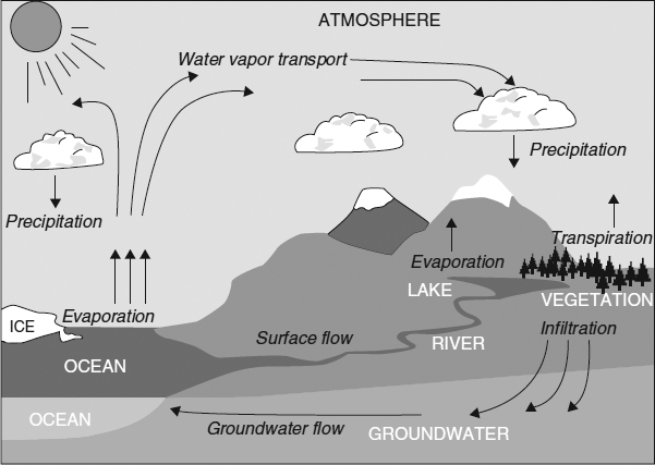
Figure 2.1 Simplified Regional Hydrologic Cycle Including Water Storage (Hydrologic Components in Capital Letters) and Exchange/Transport Processes (Items in Italics).
Source: Adapted, with permission, from Trenberth et al., 2007.
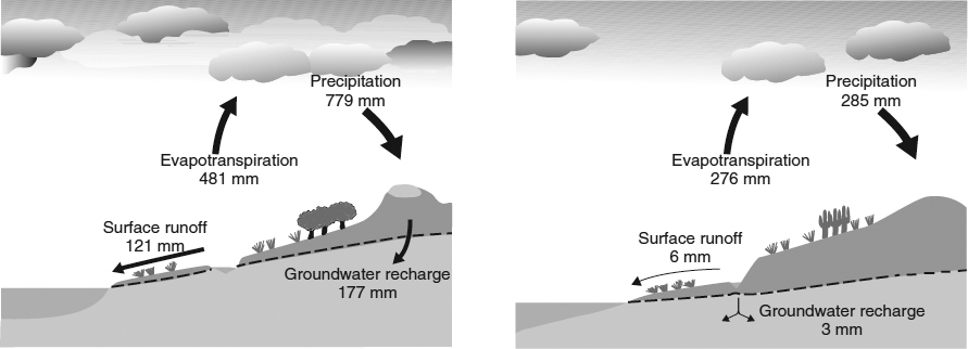
Figure 2.2 Global Variation in Hydrologic Exchanges in Germany (left) and Namibia (right). Note that values are given in millimeters of water depth. Evapotranspiration is the sum of evaporation and transpiration. When water depth is multiplied by the land area of the nation, a volume of annual water exchange is obtained. Also note that the numeric values alone may be misleading; evapotranspiration is greater in Germany than Namibia (481mm compared to 276 mm), but the relative fraction of evapotranspiration to precipitation is much greater in Namibia (276 mm/285 mm = 0.97 compared to 481 mm/779 mm = 0.62 for Germany). Note that arrow width is proportional to magnitude of transfer.
Source: Redrawn from Struckmeier et al., 2005.
The quantity and timing of water movement (exchange between components) is highly variable spatially at global (Figure 2.2), national, and regional scales. Moreover, variability exists temporally also at these same scales. For example, according to Figure 2.3, there is a large amount of variability for the Great Lakes region over the past century, with annual rainfall depths ranging from less than 25 inches to more than 40 inches.
The predicted depth and intensity of precipitation affects the design of every hydraulic component of the infrastructure (e.g., dams, levees, culverts, gutters). Rainfall storm intensities and annual depths of precipitation (Figure 2.4) vary widely across the United States. The annual average precipitation in the contiguous United States ranges from as little as a few inches per year in the arid Southwest to greater than 160 inches per year in the Pacific Northwest. Most of the United States located east of the Mississippi River experiences 30 to 50 inches of precipitation per year. This depth of precipitation is the sum of all forms (rain, snow, hail) in water equivalents, where 1 inch of rain equals 1 inch of water and 1 inch of snow may equal only 0.1 inch of water, depending on the density of the snow. In colder climates, spring snowmelt of accumulated winter precipitation can cause dramatic increases in river flows. In the arid west, reservoirs capture mountain snowmelt and store the water for use during the dry summers.
Precipitation intensity is the rate of precipitation, measured as in/hr or cm/hr.
Hydraulic components of the infrastructure are not designed based on annual average precipitation. If they were, they would be undersized 50percent of the time. Rather, hydraulic components are designed based on a selected recurrence interval. Common terminology, for example, is a “100-year storm” or “100-year drought.” This does not mean that the event will occur once every 100 years; rather, it means that the event has a 1 in 100 (1 percent) chance of occurring in any given year. Although unlikely, the 100-year storm could occur twice in a very short time; for example, Charlotte, North Carolina experienced 100-year storms in both 1995 and 1997.

Figure 2.3 Long-Term Regional Variation in Annual Precipitation in the Great Lakes Region of the Midwest.
Source: Redrawn from Hodgkins et al., 2007.

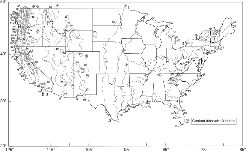
Figure 2.4 Annual Average Precipitation in the Contiguous United States.
Source: National Oceanic and Atmospheric Administration, National Climatic Data Center/Owenby et al.
Recurrence Intervals
The recurrence interval (sometimes called a “return period”) is equal to the inverse of the probability of an event happening in any given year. For example, a 10-year storm has a 1/10, or 10 percent, probability of occurring in any given year. This has many applications in infrastructure engineering, as infrastructure components need to be designed to not fail in response to a given floodwater depth, rainfall intensity, stormwater runoff, etc. A floodwall built to withstand a 100-year flood will be taller than one designed to withstand a 50-year flood. A culvert designed to convey the runoff from a 10-year storm will have a smaller diameter than the culvert designed to pass the 50-year storm. In each of these cases, the longer return period affords a lower risk and a greater sense of security but also costs more. Consequently, the infrastructure component is not expected to “handle” events that are larger than that for which it was designed. That is, a culvert designed to pass the 10-year storm is expected to “fail” (i.e., not be able to convey the runoff) for any storm larger than the 10-year storm. The failure of the culvert will lead to a flooded roadway and perhaps soil erosion and related damage to the roadway. However, if this roadway conveys minimal traffic, the selection of a 10-year storm may be appropriate given that only a few residents will be affected. (Of course, for the affected residents, this flooding may be totally unacceptable.) The recurrence interval chosen as the basis for design increases as the number of affected people and the economic risk of failure increases; for example, culverts under freeways are typically designed at the 50-year (2 percent) level.
The relationship between the storm intensity and its recurrence interval is illustrated by intensity-duration-frequency (IDF) curves (e.g., Figure 2.5). Local IDF curves are available for many regions of the country. An IDF curve is utilized when designing infrastructure components to meet desired levels of risk protection from flooding. According to an IDF curve, for a given storm duration the depth of precipitation increases as the recurrence interval increases. For example, according to the IDF curve in Figure 2.5, the 2-year intensity for a 60-minute storm duration is approximately 1.1 in/hr while the 100-year intensity for the same duration storm is approximately 2.4 in/hr.
Figure 2.5 Intensity-Duration-Frequency (IDF) Curves for Pierre, South Dakota. Note that both axes are logarithmic scale.
Source: Redrawn from South Dakota Department of Transportation.
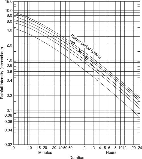

The total precipitation depth of a storm is the product of the intensity and the duration. Also as shown in Figure 2.5, for a given recurrence interval, the intensity increases as the duration decreases.
Watersheds
A watershed is the area draining (i.e., contributing runoff) to an outlet point. The outlet point may be the mouth of a river or stream, a culvert, or a stormwater inlet. When designing hydraulic structures, engineers must delineate (i.e., draw the outline or boundaries of) contributing watershed areas.
 How to Delineate a Watershed
Watershed characteristics of interest include the type of land cover (e.g., crops, forest, pavement), the soil types (e.g., sand or clay), and topography (flat, hilly, mountainous).
Columbia River Watershed
The watershed for the Columbia River is shown in Figure 2.6 (the watershed outlet being the mouth of the Columbia where it enters the Pacific Ocean). The boundaries of the watershed are mountain ridges; for example, precipitation falling west of the watershed boundary in Montana will travel to the Columbia River, whereas precipitation east of the watershed boundary (in the adjacent watershed of the Missouri River) will travel to the Gulf of Mexico. Notice that the Columbia River watershed is contained within seven states and one Canadian province of British Columbia, making management of the river quite challenging. The Columbia River has many tributaries (rivers feeding into it). Each of them has its own watershed, which is considered a sub-watershed of the Columbia River. The largest sub-watershed, the Snake River watershed, is delineated with a dashed line in Figure 2.6; the outlet is the confluence of the Snake and Columbia Rivers. The Snake River also has many sub-watersheds for each of its tributaries.
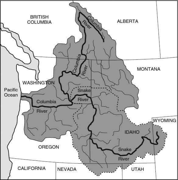
Figure 2.6 The Columbia River Watershed (Shaded Area) and Its Largest Sub-Watershed (Snake River, Delineated by Dashed Line).

Figure 2.7 Map of Major U.S. Watersheds. The Mississippi River basin is delineated in dark blue.
Source: U.S. Geological Survey.
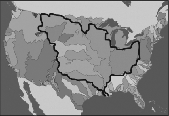
Major watersheds in the United States are mapped in Figure 2.7. The Mississippi River watershed, one of the largest in the world, is outlined with a dark solid line. This basin (large watershed) includes the watersheds of the Missouri River, the Ohio River, the Arkansas River, and many other major rivers. Knowing the boundaries of this watershed aids in managing the quality and quantity of water in the Mississippi River. For example, knowing the contributing area is necessary in predicting floods for various reaches of the river. Also, predicting the mass of pollutants, such as sediment and nutrients, entering the Gulf of Mexico can be accomplished by mathematical modeling of the river and its watershed and sub-watersheds.
As used in this text, the term “mathematical model,” or often simply “model,” refers to a collection of mathematical expressions or formulae that predict how systems, both natural and built, will behave.
Rivers
Because of complexities such as soil infiltration rates, snow melt, and the varying travel times of storm runoff to rivers, a 100-year storm does not necessarily result in a 100-year flood. Rather, flood probabilities are based on long-term measurements of actual river stage (water elevation), rather than precipitation. An example of such historic data is provided in Figure 2.8.

Figure 2.8 Maximum Annual River Stage (Elevation) for the Susquehanna River at Williamsport, Pennsylvania. Note that data has been collected at this site for more than 100 years. The record stage of 35 feet occurred in 1972 when Hurricane Agnes produced 18 inches of rain over a 5-day period.
Source: U.S. Geological Survey.
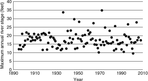
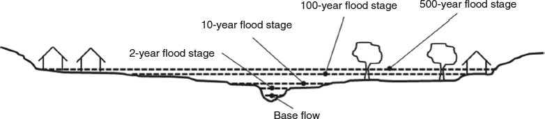
Figure 2.9 Cross-Section View of a River and Floodplain Valley.
A cross-section of a river and floodplain can be seen in Figure 2.9, with several flood stages noted. In Figure 2.9, base flow is identified, which corresponds to the “normal” water depth for the river at times between substantial runoff events. For runoff events with recurrence intervals greater than 2 years, the depth of water will be higher than the top of the riverbank, and given the topography of the land, this water will spread laterally across the floodplain to a land elevation equal to the water depth. Figure 2.10 is a plan (aerial) view of this same floodplain and the extents of the 100-year and 500-year floods.
A floodplain is the land along a stream or river that is inundated when the stream or river overtops its banks.
The 100-year floodplain is especially noteworthy, given that most modern building codes prohibit building permanent structures in the 100-year flood-plain. The delineation of the floodplain is provided by the National Flood Insurance Program of the Federal Emergency Management Agency (FEMA). Many older structures, including homes, are located in the 100-year flood-plain. This may be because the homes are very old and were built before floodplain maps were available. Also, consider a home that was built along a river for which flooding is minimized by an upstream dam. If the dam is removed, the boundary of the 100-year floodplain will change substantially.
Alternatively, as a watershed becomes increasingly developed with more impervious surfaces (paved parking lots, roads, and rooftops that limit infiltration), more runoff occurs for any given storm event. Thus, the flood stage for any recurrence interval tends to increase over time. For flood insurance and development planning reasons, FEMA is updating floodplain maps to more accurately delineate current flood zones. This is an important, challenging, and expensive endeavor, costing more than $1 billion, and will utilize mathematical models and data collected by engineers and scientists.
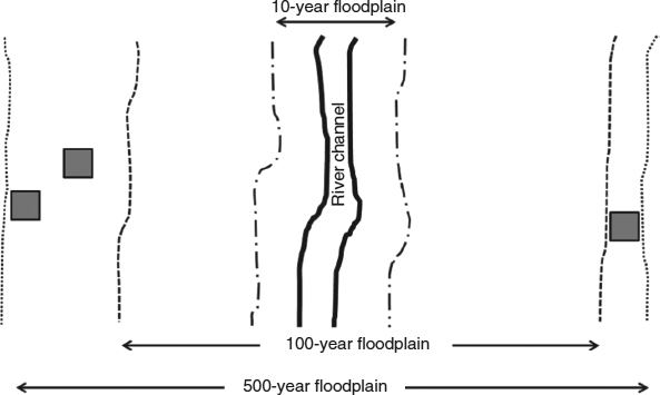
Figure 2.10 Aerial (Plan) View of River and Valley from Figure 2.9. Note that the homes (squares) are located outside of the 100-year floodplain as required by building codes.
The Fickle Power of Nature
Rivers and streams create their own routes, which move over time. Site investigations have shown that some river channels have moved laterally by as much as 100 feet in the last two centuries. Many civil engineering projects have tried (often successfully, sometimes not) to “contain” rivers to a desired path. Consideration of the tendency for river channels to migrate is important when infrastructure projects are located near rivers (e.g., choosing bridge locations; see Figure 2.11).
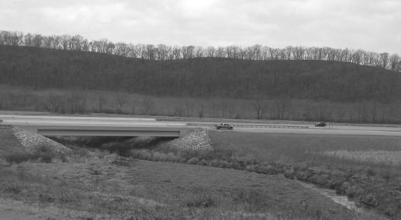
Figure 2.11 Armored Bridge Abutments. Note the armoring of bridge abutments with rip-rap (6 inches to 18 inches in size) used to prevent scour during flood stages. Also note that construction of this particular bridge required the filling of wetlands in the floodplain.
Source: M. Penn.
Habitat/Native Species
Development inherently eliminates wildlife habitat and otherwise affects the natural environment; however, it is possible to minimize habitat loss by controlling the location or type of development. Many community and regional planning organizations identify rare or important natural resources and prevent or discourage development in those areas. Federal and state regulations also limit development in areas documented as habitat for endangered species. Some types of development can include green space that can be designed to provide wildlife habitat. Designing a functioning habitat depends on the species desired, and is not as simple as planting a few trees and shrubs. Professionals, most likely without engineering backgrounds, that have training and experience in habitat design should be consulted.
Wetlands
Wetlands are often viewed as “stumbling blocks” to many development and transportation projects due to their highly regulated nature. Such regulations are necessary, given that in the past 150 years, more than half of U.S. wetlands have been drained or filled for urban, suburban, and agricultural uses. Wetlands provide many potential benefits ranging from recreational activities to floodwater storage. Some wetlands provide habitat for rare or endangered plants and wildlife.
The Use of Native Species
The use of native species of plants has gained popularity from an aesthetic and ecological landscaping perspective. In some cases, local or state regulations recommend or require the use of native plant species. For example, prairies, with very diverse grasses and flowers, once ranged from the Great Plains to the Midwest prior to settlement and subsequent conversion to agriculture. Some states have begun planting thousands of acres of native prairie plants along highway roadsides (Figure 2.12). Native plants offer the advantages of being best suited (i.e., naturally selected) for the climate at the site location, reducing erosion, increasing water infiltration, and offering natural microhabitats. In addition, during the summer and fall bloom period, the wildflowers greatly enhance the beauty of the roadside.
Roadsides for Wildlife brochure, Minnesota Department of Natural Resources
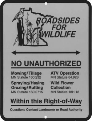
Figure 2.12 A Roadside Prairie Sign.
Source: Minnesota Department of Natural Resources.
Wetlands, by legal definition, are not necessarily always “wet” (i.e., containing ponded water). When you think of a wetland, you may envision a swampy area or a marsh with ducks and cattails. Indeed, these examples are classified as wetlands. But many types of wetlands do not fit this stereotypical view of a wetland (Figure 2.13).
Proper identification and location of wetlands is critical at development sites, and is accomplished using wetland delineation. Failure to identify a wetland may lead to costly fines and potential project delays. Definitions vary at the local, state, and federal level, but in general, wetlands are areas that have, for a significant portion of the plant growing season, groundwater within a few feet of the ground surface or ponded water at the ground surface. This definition stems from the fact that certain plants and the wildlife that depend upon them, flourish in wet soils, whereas other plants do not.
Trained scientists and engineers evaluate the hydrology, soils, and plants at a site to determine whether or not a wetland exists and to determine its spatial extent (termed wetland delineation).
Wetlands will be discussed in more detail in Chapter 15, Environmental Considerations.
Geologic Formations
Having an understanding of geologic formations is necessary to understand groundwater flow, infiltration, and runoff. Such understanding is also necessary for designing rock cuts for roads and foundations for buildings. Additionally, geologic formations are sources of building materials for roads, levees, and other infrastructure components.
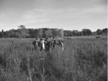
Figure 2.13 Students Learning to Identify Wetland Plants and Soils in a “Wet Prairie.” There is no “standing” water typically in this type of wetland.
Source: M. Penn.
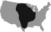
Soil is the uppermost (surface) layer of unconsolidated material that lies above the uppermost layer of rock (consolidated material), termed bedrock. Soil is the biologically active upper layer of unconsolidated material and may range from approximately 2 to 20 feet in depth below the surface. The biologically inactive unconsolidated material below soil is termed subsoil. The depth of unconsolidated material varies based on how it was deposited (e.g., by wind or by glacier) and on the shape of the bedrock surface below; this surface may be “uneven” due to prior geologic occurrences (e.g., an ancient river gorge). The depth of unconsolidated material can vary dramatically over small distances or in some cases can be very uniform over large distances. Figure 2.14 is a depth to bedrock map for Stearns County, Minnesota. Based on our definitions of bedrock and unconsolidated material, we could also describe Figure 2.14 as a map of the thickness of the unconsolidated material. Note that in the southwest corner of the county, over a distance of only approximately 15 miles, the depth of unconsolidated material ranges from less than 100 feet to nearly 500 feet, which demonstrates the need for proper geotechnical site investigations for any project.
Unconsolidated material refers to loosely arranged organic and mineral particles that are not cemented together.

For example, at the University of Wisconsin-Platteville (the authors' campus), a new building was planned for construction. The initial site investigation included several borings to locate the bedrock depth for designing the building's foundation (Figure 2.15). Based on the results of the borings, engineers predicted a bedrock surface, and used the depth of this predicted surface when designing the foundation and estimating the cost of excavation. However, when excavation commenced, bedrock was encountered at shallower depths than expected in some areas between the locations of the borings (Figure 2.16). The project was delayed and additional costs were incurred because of the additional unanticipated blasting and excavating.
Borings are vertically drilled holes used to identify geologic materials present at various depths.
In some locations across the United States, the bedrock represents a massive formation which may extend vertically for thousands of feet. In other areas, many layers of rock exist, as is evident for the cross-section of Kansas provided in Figure 2.17. Each layer has different properties that can affect engineering decisions. These properties include bedrock strength, which will affect the design of foundations, and the porosity and extent of fractures, which will affect groundwater flow.
Porosity is a measure of the void spaces in a geologic formation. Porosity is equal to the volume of void spaces in the sample divided by the total sample volume. For example, some types of sandstone have porosities of 0.1; thus, a 1 cubic foot of sample of sandstone would contain 0.1 cubic feet of void space and 0.9 cubic feet of sand.
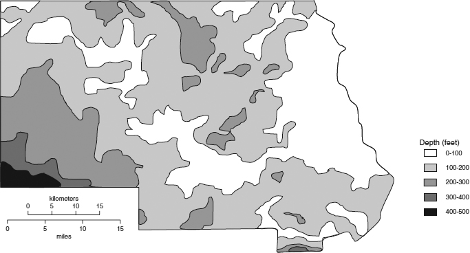
Figure 2.14 Depth to Bedrock (or Thickness of Unconsolidated Material) in Stearns County, Minnesota.
Source: Redrawn from Minnesota Geological Survey.
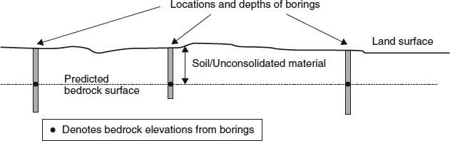
Figure 2.15 Location of Borings and Predicted Bedrock Elevations (Dotted Line) for a Building Foundation.
Groundwater flow, like many natural processes, is typically hidden from view. One case in which groundwater flow can be observed is depicted in Figure 2.18. Groundwater is seeping out between layers of rock. In this instance, the groundwater preferentially flows outward in the horizontal direction as compared to downward in the vertical direction. In general, large fractures or highly porous formations favor groundwater flow, while impermeable formations hinder groundwater flow. The “icicles” in the photo form at the openings of vertical fractures.
While you may think of the earth's crust (the uppermost rock layers, tens of thousands of feet in thickness) as a stable body, it is not. Movement of geologic formations creates stress that can cause large planar fractures, or faults. Sudden movement along faults is the cause of seismic activity (earthquakes), which varies in magnitude from undetectable to catastrophic. Earthquakes occur continuously, literally hundreds across the globe in any given week.
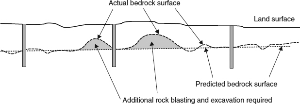
Figure 2.16 Predicted and Actual Bedrock Surface, and Additional Rock Removal Required.
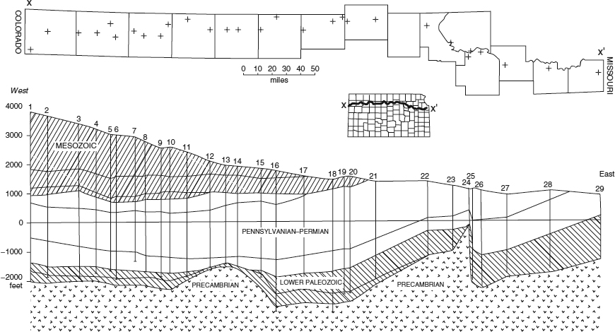
Figure 2.17 Geologic Cross-Section of the State of Kansas Illustrating Sedimentary Rock Layers. Note the exaggerated vertical scale. Names refer to geologic periods of deposition. Numbers and vertical lines in cross-section correspond to borings at locations marked (+) in plan view.
Source: Redrawn from Merriam and Hambleton.


Figure 2.18 Observation of Groundwater Flow. (a) Icicles forming on the face of a roadcut from horizontal groundwater seepage along the top of a rock layer (darker formation shown with arrow) that is more restrictive to vertical flow. (b) Cross-sectional view of the geologic formations shown in the photo. The shaly dolomite layer is more restrictive to vertical groundwater migration than the other rock types, but some water does pass through to recharge the groundwater table. Arrows are scaled by width (not length) to represent the relative amount of groundwater flow. Note that the groundwater table (defined in the next section) is below the elevation of the roadway.
Source: M. Penn.

Figure 2.19 Damage Caused by the 1989 San Francisco Earthquake.
Source: U.S. Geological Survey.
The “Bay Area” of California (San Francisco, Oakland, and San Jose), one of the 10 largest metropolitan areas in the country, is located on and near more than one dozen major faults. In 1906, an earthquake here killed more than 3,000 people in what is considered one of the worst natural disasters in our nation's history. In 1989, another earthquake caused an estimated $6 billion in damages (Figure 2.19) and claimed more than 60 lives. The decreased number of fatalities can be in part attributed to the lesser magnitude of the 1989 earthquake (6.9 as compared to 7.9 on the Richter scale); however, credit must also be given to the work of civil and environmental engineers—both in the design of earthquake-resistant structures and in the development of infrastructure that allows speedy emergency response. An effective infrastructure also allows for a relatively rapid recovery and less disruption to daily lifestyles, while, as witnessed by the recent Haiti earthquake (Figure 2.20), an infrastructure-poor country takes much longer to recover.

Map of Latest Earthquakes in the World—Past 7 Days, U.S. Geological Society.
While California and Alaska experience the most earthquakes, damaging earthquakes have occurred across the United States. Many geotechnical and structural engineers specialize in designing foundations and structures that can withstand seismic activity.
Many civil and environmental engineering programs require a course in geology or geomorphology. Understanding geologic formations and processes is vital to infrastructure engineering.
Geomorphology is the study of landforms and the processes that shape them.
Groundwater
Water is found in the subsurface in pores of unconsolidated material and in pores and fractures in rock. Below the water table, or groundwater table, all pores and fractures are filled with water. The depth to the water table from the ground surface may range from zero in a wetland to hundreds of feet (Figure 2.21).
The water table occurs at the depth at which the geologic formation is saturated.
An aquifer is a geologic formation that stores water. Aquifers may be shallow (less than 100 feet below ground surface) or deep (sometimes greater than 1,000 feet below ground surface) and are composed of granular unconsolidated material, of fractured bedrock, or of porous rock (e.g., sandstone). Water is extracted from aquifers by drilling a well (a vertical borehole in the ground) and pumping the water out of the well. Groundwater availability is highly variable across the United States. Where it is plentiful enough to meet large water demands, groundwater is used for public drinking water systems and industries. In regions where it is not economically feasible to extract groundwater, surface waters are used for water supply. Most rural residences have individual private drinking water wells as the small demands required can readily be obtained.
Figure 2.20 Aftermath of Haiti Earthquake.
Source: Copyright © Claudia Dewald/iStockphoto.
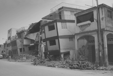
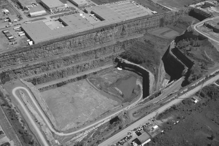
Figure 2.21 An Aerial View of an Operating Limestone Quarry. Quarry excavation typically continues downward until the water table is reached, which has yet to occur in this quarry. In this case, the water table is greater than 150 feet below ground surface. The dark area in the center of the photo is a stormwater pond at the lowest elevation to collect stormwater runoff. Note the minimal setback distance (approximately 30 feet) from open excavation to the industrial building in the background; such a short setback is allowed because of the stability of the geologic formation.
Source: Copyright © Yvan Dubé/istockphoto.
One important characteristic of groundwater can be understood by applying a hydrologic budget to an aquifer. As development occurs, previously pervious areas are made impervious by paving driveways and roads and by constructing rooftops. As a result, more runoff occurs and there is a corresponding decrease in infiltration to groundwater (termed recharge). Consequently, the mass of water stored in aquifers decreases and groundwater levels are lowered. This may lead to decreased stream flows in streams that are fed by groundwater, and to the unwanted conversion of wetlands to “drylands.” Similarly, pumping groundwater out of an aquifer at a rate that is greater than the natural rate of recharge will lower groundwater levels.
Many public water supplies that rely on groundwater are finding that groundwater levels are dropping, sometimes at the rate of several feet per year. This is not only occurring in the arid southwestern states, but throughout the country. As a result, groundwater must be pumped up from lower depths, resulting in more costly pumping and possibly the installation of deeper wells if deeper aquifers exist. If no other aquifers are present, alternative water supplies must be identified, often at great expense (e.g., by damming a river).
Atmosphere
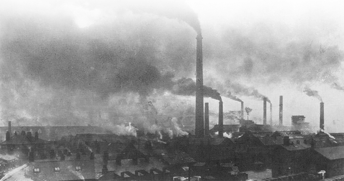
The atmosphere is the major transport mechanism for water in the hydrologic cycle, and has complex interrelationships with the land surface and oceans with respect to global climate change (discussed in the following section). Air quality primarily deals with the air that we breathe in the lower atmosphere (stratosphere) and the potential adverse health effects of pollution (Figure 2.22). However, air quality also deals with aesthetics (visibility) and degradation of structures (e.g., acid rain). Furthermore, many pollutants cycle between land, water, and air. Some types of air pollution are linked to degraded surface water quality, and thus human and wildlife health via contaminated fish consumption. Interactions between infrastructure and air quality will be discussed throughout this book.
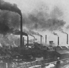
Figure 2.22 Air Quality in Widnes, England, in the Late 1800s was Typical of Industrial Cities in the United States. Due to passage of the Clean Air Act of 1970 and the 1990 Amendment, air quality is much better today. However, air quality remains a public health concern in many urban areas.
Source: Wikipedia: http://commons.wikimedia.org/wiki/File:Widnes_Smoke.jpg.
Climate Change
Human-induced climate change (i.e., global warming) has been debated for decades by scientists, policymakers, and the public. Greenhouse gases (carbon dioxide, methane, nitrous oxide, ozone, and others) have been rapidly accumulating in our atmosphere (Figure 2.23) and trap heat radiating outward from the earth. A common analogy for the greenhouse effect is a car with the windows shut on a sunny day—light (short wavelength radiation) enters through the glass and is converted into heat (long wavelength radiation), which is trapped by the glass.
In 1990, the Intergovernmental Panel on Climate Change (IPCC) released its first report on climate change which, along with subsequent reports, led to the Kyoto Agreement for greenhouse gas emission reductions. Nearly 200 nations have signed the protocol; the United States, the second largest CO2 emitter (recently surpassed by China), has yet to agree to the requirements at the time of writing of this textbook. The IPCC's claim that the major cause of recent (last 50 years) global warming is very likely to be anthropogenic (human induced) is supported by the national science academies of nearly all industrialized nations and is now considered to be scientific consensus. There is, however, debate as to the extent of this relationship relative to naturally occurring warming processes.
The potential negative consequences of climate change typically intensify with increasing temperature rise. The consequences are vast (Parry et al., 2007), and often regional, including:
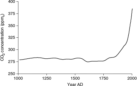
Figure 2.23 Increases in CO2 Gas Concentrations in the Atmosphere Over the Past 1,000 Years. Although not shown, the trends for nitrous oxide and methane are similar. Data prior to 1950 is based on ice cores while data since 1955 is based on atmospheric measurements.
Data source: Carbon Dioxide Information Analysis Center.
- Increased drought, leading to decreased water availability for hundreds of millions of people
- Increased risk of species extinction
- Loss of coral reefs
- Changes in global carbon cycling
- Shifts in suitable habitat for species
- Increased wildfire risk
- Changes in suitability for crop production
- Increased flooding
- Loss of coastal wetlands
- Increased malnutrition and disease
Complex mathematical climate models not only estimate averaged global temperature, but also regional temperature and weather pattern changes. Some models predict more intense rainstorms, tornadoes, and hurricanes, all of which potentially have disastrous effects on the built and natural environments.
Because of melting glaciers and polar ice caps, sea levels are expected to rise. Estimates range from 8 inches to 20 inches over the next century above current levels (Figure 2.24). To the untrained engineer, this might not seem significant, but it is potentially very significant. If flood protection systems are overtopped, flooding will occur. And given that there have been many cases where floodwaters have come within inches of overtopping levees (e.g., Figure 2.25), a few additional inches of sea level increase could have catastrophic results.
U.S. Army Corps of Engineers Circular on Incorporating Sea Level Change in Civil Works
In 2009, the U.S. Army Corps of Engineers adopted a policy whereby future sea level predictions must be incorporated in to the planning and design of all of its projects. “To ignore rising sea level in the design of civil works would be like ignoring the health effects of smoking a cigarette … we've gotten to that point,” Jim Titus, a U.S. Environmental Protection Agency researcher, said, in response to the release of the policy (Luntz, 2009). Adaptive management is an increasingly common and effective approach to deal with future uncertainties of all kinds. For example, without adaptive management, two options exist for a new levee: (1) design the levee for the expected future floodwater elevation, or (2) design an even taller levee for protection against potentially higher floodwaters, which may or may not occur. In the first case, if future floodwaters are indeed higher than expected, the cost to raise the levee will be significant. In the second case, the taller levee would be more expensive to design and build, and would be unnecessary if higher floodwaters do not occur. With adaptive management, a “middle ground” can be achieved. A levee design can specify a levee that will contain expected floodwater elevations and that can be readily modified as warranted by future circumstances. In this case, since the initial design accounted for the future possibility of raising the levee, the cost to raise the levee would be less than retrofitting a levee that was not designed to accommodate modification.
Adaptive management is a process whereby future uncertainties are incorporated into a plan or design so that if changes do occur, a strategy is already in place to deal with them.
Figure 2.24 Historical and Projected Range of Sea Level Rise. Note that scale is in millimeters (100 mm ≈ 4 inches). Actual instrumental measurements have been made since 1870. Prior to this date, estimates are made by a variety of scientific techniques.
Source: U.S. Environmental Protection Agency.
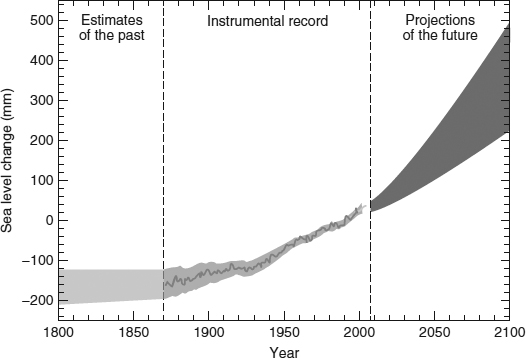

Figure 2.25 One of the Authors Holds a 1996 Newspaper Published the Day After a Flood Crest Nearly Overtopped the Levees (Over Which the Bridge in the Photo Passes) in Wilkes-Barre, Pennsylvania. The Susquehanna River level rose 30 feet in a 2-day period following a 2-inch rainstorm and warm weather causing excessive snowmelt in January.
Source: M. Penn.

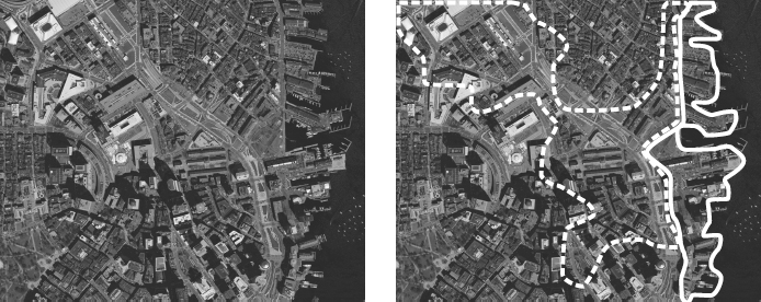
Figure 2.26 Downtown Boston (left) and 100-Year Flood Zones (right). The existing flood zone is depicted by the solid line. The predicted future flood zones corresponding to a “high level” of greenhouse gas emissions scenario, is depicted by the dashed line.
Source: U.S. Geological Survey, and floodplain boundaries adapted from Frumhoff et al., 2007.
![]() Remember that full-sized versions of textbook photos can be viewed in color at www.wiley.com/college/penn.
Remember that full-sized versions of textbook photos can be viewed in color at www.wiley.com/college/penn.
Sea level rise is of particular concern for coastal communities such as Boston, Massachusetts (Figure 2.26), many of which have experienced rapid growth in recent years.

Outro
The natural environment supports all life and, in many different ways, all infrastructure. Human activity and infrastructure development has many potential adverse effects on the land, water and air. The impact of infrastructure on the environment and the impact of the environment on infrastructure must be fully understood in order to plan and design future growth that is sustainable.
chapter Two Homework Problems
- 2.1 Use Figure 2.24 to estimate low-range and high-range projected rates of sea level rise (mm/yr) from 2010 to 2100. Convert these rates to inches per year. Show all work.
- 2.2 For Pierre, South Dakota (Figure 2.5), what is the precipitation intensity of a storm that:
- lasts 10 minutes, given a recurrence interval of 100 years?
- lasts 30 minutes, given a recurrence interval of 10 years?
- lasts 30 minutes, given a recurrence interval of 2 years?
- lasts 2 hours, given a recurrence interval of 10 years?
- 2.3 Using Figure 2.5, calculate precipitation depth for a 3-hour duration event with the following probabilities of occurrence in a given year:
- 1%
- 10%
- 50%
- 2.4 One million gallons per day (MGD) infiltrates into an aquifer.
- If 1.05 MGD are extracted from the aquifer, by how many gallons will the aquifer be depleted in one year?
- If 1.05 MGD are extracted from the aquifer, but development has caused the infiltration rate to drop to 0.95 MGD, how does this change in infiltration change your answer from part “a”?
- 2.5 A pond has a surface area of 1.0 acre. A stream flows into the pond at a steady flowrate of 1.20 cfs (cubic feet per second) for the entire year. The evaporation rate, also steady for the entire year, is 1 inch/month. Assume that the pond is circular and has straight sides (that is, it has the shape of a cylinder). The pond has no outflow stream but a farmer withdraws water for 4 months of the year at a rate of 3.50 cfs.
- What annual change in pond volume (ft3) corresponds to the evaporation rate of 1 inch/month? That is, what volume of water evaporates in one year?
- What is the annual change in storage in the pond, in ft3, due to all inflows and outflows? Use the relationship that volume is the product of flowrate and time, and convert all values to the same units.
- What is the change in water depth for one year?
- 2.6 Given that Germany has a land area of 349,520 km2 and Namibia has a land area of 824, 290 km2, the volume associated with the hydrologic exchanges in Figure 2.2 can be calculated as the product of land area (km2) and hydrologic exchange (mm).
- Create a table that compares the volume of surface water runoff, precipitation, evapotranspiration, and groundwater recharge for Namibia and Germany. Present your answers with units of m3.
- Apply Equation 2.1 to the land surface of each of these countries and comment on the change in storage that you calculate.
- 2.7 What is the difference between soil and unconsolidated material?
- 2.8 What are the components and transfer mechanisms of the hydrologic cycle?
- 2.9 Why are many existing homes located in floodplains?
- 2.10 What are some advantages to using native species in plantings?
- 2.11 What are some benefits that wetlands provide?
- 2.12 How does the development of land affect aquifers?
- 2.13 What are some possible outcomes of the failure to incorporate climate change in long-term infrastructure planning?
- 2.14 What are the possible outcomes if infrastructure planning and design accounts for climate change but scientific predictions are incorrect and temperatures do not increase as expected?
- 2.15 Find information on the depth of water supply wells and the associated geologic formations for a community of your choice. Your state's Department of Natural Resources (sometimes named Environmental Protection Agency or Department of Environmental Conservation) website might be a good place to start.
- 2.16 Delineate the watershed in which your university is located. Is this a sub-watershed of a larger basin? A topographic map may be downloaded from a variety of websites such as msrmaps.com.
Key Terms
- adaptive management
- air quality
- aquifer
- base flow
- basin
- bedrock
- borings
- consolidated material
- delineate
- evaporation
- floodplain
- geomorphology
- hydrologic budget
- hydrologic cycle
- impervious
- infiltration
- intensity of precipitation
- mathematical modeling
- porosity
- recharge
- recurrence interval
- rip-rap
- runoff
- soil
- stage
- subsoil
- transpiration
- unconsolidated material
- water table
- watershed
- wetland delineation
References
Carbon Dioxide Information Analysis Center. http://cdiac.ornl.gov/ftp/trends/co2/lawdome.combined.dat, accessed August 6,2011.
Frumhoff, P. C., J. J. McCarthy, J. M. Melillo, S. C. Moser, and D. J. Wuebbles. 2007. Confronting Climate Change in the U.S. Northeast: Science, Impacts, and Solutions. Cambridge, MA: Union of Concerned Scientists.
Hardie, D. W. F. 1950. A History of the Chemical Industry in Widnes. Imperial Chemical Industries Limited.
Hodgkins, G. A., R. W. Dudley, and S. S. Aichele. 2007. Historical Changes in Precipitation and Streamflow in the U.S. Great Lakes Basin, 1915-2004. USGS Scientific Investigations Report 2007-5118.
Luntz, T. 2009. “New Army Corps Policy Forces Project Designers to Consider Rising Seas.” New York Times. November 11,2009.
Merriam, D. F., and W. W. Hambleton. 1959. “Relation of Magnetic and Aeromagnetic Profiles to Geology in Kansas”; in, Symposium on geophysics in Kansas: Kansas Geological Survey, Bull. 137, pp. 153-173.
Minnesota Geological Survey. Geologic Atlas of Stearns County Minnesota, C-10, Part A, Plate 5, Depth to Bedrock.
Owenby, J., R. Heim, Jr., M. Burgin and D. Ezell. Climatography of the U.S. No. 81—Supplement # 3, Maps of Annual 1961-1990 Normal Temperature, Precipitation and Degree Days. http://www.ncdc.noaa.gov/oa/documentlibrary/clim81supp3/clim81.html, accessed August 6, 2011.
Parry, M. L., O. F. Canziani, J. P. Palutikof, P. J. van der Linden, and C. E. Hanson, Eds. 2007. Climate Change 2007: Impacts, Adaptation and Vulnerability. Cambridge, UK: Cambridge University Press.
South Dakota Department of Transportation. Road Design Manual. http://www.sddot.com/pe/roaddesign/plans_rdmanual.asp, accessed August 6, 2011.
Struckmeier, W., Y. Rubin, and J. A. A. Jones. 2005. Groundwater: Reservoir for a Thirsty Planet? Earth Sciences for Society Foundation, Leiden, The Netherlands. http://www.yearofplanetearth.org/content/downloads/Groundwater.pdf, accessed August 6, 2011.
Trenberth, K. E., L. Smith, T. Qian, A. Dai and J. Fasullo. 2007. “Estimates of the Global Water Budget and its Annual Cycle Using Observational and Model Data.” Journal of Hydrometeorology, 8: 758-769.
United States Environmental Protection Agency. Seal Level Rise Projections to 2100. http://www.epa.gov/dimatechange/science/futureslc_fig1.html, accessed August 6, 2011.
United States Geological Survey, USGS Gauging station 01551500 (WB Susquehanna River at Williamsport).