Chapter Four. Algorithms and Data Structures

This chapter presents fundamental data types that are essential building blocks for a broad variety of applications. This chapter is also a guide to using them, whether you choose to use Java library implementations or to develop your own variations based on the code given here.

Objects can contain references to other objects, so we can build structures known as linked structures, which can be arbitrarily complex. With linked structures and arrays, we can build data structures to organize information in such a way that we can efficiently process it with associated algorithms. In a data type, we use the set of values to build data structures and the methods that operate on those values to implement algorithms.

The algorithms and data structures that we consider in this chapter introduce a body of knowledge developed over the past 50 years that constitutes the basis for the efficient use of computers for a broad variety of applications. From n-body simulation problems in physics to genetic sequencing problems in bioinformatics, the basic methods we describe have become essential in scientific research; from database systems to search engines, these methods are the foundation of commercial computing. As the scope of computing applications continues to expand, so grows the impact of these basic methods.

Algorithms and data structures themselves are valid subjects of scientific study. Accordingly, we begin by describing a scientific approach for analyzing the performance of algorithms, which we apply throughout the chapter.

To study the cost of running them, we study our programs themselves via the scientific method, the commonly accepted body of techniques universally used by scientists to develop knowledge about the natural world. We also apply mathematical analysis to derive concise mathematical models of the cost.

Which features of the natural world are we studying? In most situations, we are interested in one fundamental characteristic: time. Whenever we run a program, we are performing an experiment involving the natural world, putting a complex system of electronic circuitry through series of state changes involving a huge number of discrete events that we are confident will eventually stabilize to a state with results that we want to interpret. Although developed in the abstract world of Java programming, these events most definitely are happening in the natural world. What will be the elapsed time until we see the result? It makes a great deal of difference to us whether that time is a millisecond, a second, a day, or a week. Therefore, we want to learn, through the scientific method, how to properly control the situation, as when we launch a rocket, build a bridge, or smash an atom.

On the one hand, modern programs and programming environments are complex; on the other hand, they are developed from a simple (but powerful) set of abstractions. It is a small miracle that a program produces the same result each time we run it. To predict the time required, we take advantage of the relative simplicity of the supporting infrastructure that we use to build programs. You may be surprised at the ease with which you can develop cost estimates and predict the performance characteristics of many of the programs that you write.

• Observe some feature of the natural world.

• Hypothesize a model that is consistent with the observations.

• Predict events using the hypothesis.

• Verify the predictions by making further observations.

• Validate by repeating until the hypothesis and observations agree.

One of the key tenets of the scientific method is that the experiments we design must be reproducible, so that others can convince themselves of the validity of the hypothesis. In addition, the hypotheses we formulate must be falsifiable—we require the possibility of knowing for sure when a hypothesis is wrong (and thus needs revision).

Our first qualitative observation about most programs is that there is a problem size that characterizes the difficulty of the computational task. Normally, the problem size is either the size of the input or the value of a command-line argument. Intuitively, the running time should increase with the problem size, but the question of by how much it increases naturally arises every time we develop and run a program.

Another qualitative observation for many programs is that the running time is relatively insensitive to the input itself; it depends primarily on the problem size. If this relationship does not hold, we need to run more experiments to better understand the running time’s sensitivity to the input. Since this relationship does often hold, we focus now on the goal of better quantifying the correspondence between problem size and running time.

As a concrete example, we start with ThreeSum (PROGRAM 4.1.1), which counts the number of (unordered) triples in an array of n numbers that sum to 0 (assuming that integer overflow plays no role). This computation may seem contrived to you, but it is deeply related to fundamental tasks in computational geometry, so it is a problem worthy of careful study. What is the relationship between the problem size n and the running time for ThreeSum?

• Detailed understanding of the program

• Detailed understanding of the system and the computer

• Advanced tools of mathematical analysis

Thus, it is best left for experts. Every programmer, however, needs to know how to make back-of-the-envelope performance estimates. Fortunately, we can often acquire such knowledge by using a combination of empirical observations and a small set of mathematical tools.

public class ThreeSum
{
   public static void printTriples(int[] a)
   {  /* See Exercise 4.1.1. */  }

   public static int countTriples(int[] a)
   {  // Count triples that sum to 0.

      int n = a.length;
      int count = 0;
      for (int i = 0; i < n; i++)
         for (int j = i+1; j < n; j++)
            for (int k = j+1; k < n; k++)
               if (a[i] + a[j] + a[k] == 0)
                  count++;
      return count;
   }

   public static void main(String[] args)
   {
      int[] a = StdIn.readAllInts();
      int count = countTriples(a);
      StdOut.println(count);
      if (count < 10) printTriples(a);
   }
}

   n   | number of integers
  a[]  | the n integers
 count | number of triples that sum to 0

% more 8ints.txt
 30
-30
-20
-10
 40
  0
 10
  5

% java ThreeSum < 8ints.txt
4
 30 -30   0
 30 -20 -10
-30 -10  40
-10   0  10

% java ThreeSum < 1Kints.txt
0

• The cost of executing each statement

• The frequency of executing each statement

The former is a property of the system, and the latter is a property of the algorithm. If we know both for all instructions in the program, we can multiply them together and sum for all instructions in the program to get the running time.

The primary challenge is to determine the frequency of execution of the statements. Some statements are easy to analyze: for example, the statement that sets count to 0 in ThreeSum.countTriples() is executed only once. Other statements require higher-level reasoning: for example, the if statement in ThreeSum.countTriples() is executed precisely n (n–1)(n–2)/6 times (which is the number of ways to pick three different numbers from the input array—see EXERCISE 4.1.4).

public class DoublingTest
{
   public static double timeTrial(int n)
   {  // Compute time to solve a random input of size n.
      int[] a = new int[n];
      for (int i = 0; i < n; i++)
         a[i] = StdRandom.uniform(2000000) - 1000000;
      Stopwatch timer = new Stopwatch();
      int count = ThreeSum.countTriples(a);
      return timer.elapsedTime();
   }

   public static void main(String[] args)
   {  // Print table of doubling ratios.
      for (int n = 512; true; n *= 2)
      {  // Print doubling ratio for problem size n.
         double previous = timeTrial(n/2);
         double current  = timeTrial(n);
         double ratio = current / previous;
         StdOut.printf("%7d %4.2f
", n, ratio);
      }
   }
}

   n   | problem size
  a[]  | random integers
 timer | stopwatch

    n    | problem size
previous | running time for n/2
 current | running time for n
  ratio  | ratio of running times

% java DoublingTest
    512 6.48
   1024 8.30
   2048 7.75
   4096 8.00
   8192 8.05
  ...

Frequency analyses of this sort can lead to complicated and lengthy mathematical expressions. To substantially simplify matters in the mathematical analysis, we develop simpler approximate expressions in two ways.

First, we work with only the leading term of a mathematical expression by using a mathematical device known as tilde notation. We write ∼f (n) to represent any quantity that, when divided by f (n), approaches 1 as n grows. We also write g (n)∼f (n) to indicate that g (n) / f (n) approaches 1 as n grows. With this notation, we can ignore complicated parts of an expression that represent small values. For example, the if statement in ThreeSum is executed ∼n³/6 times because n (n–1)(n–2)/6 = n³/6 – n²/2 + n/3, which certainly, when divided by n³/6, approaches 1 as n grows. This notation is useful when the terms after the leading term are relatively insignificant (for example, when n = 1,000, this assumption amounts to saying that –n²/2 + n/3 ≈ –499,667 is relatively insignificant by comparison with n³/6 ≈ 166,666,667, which it is).

Second, we focus on the instructions that are executed most frequently, sometimes referred to as the inner loop of the program. In this program it is reasonable to assume that the time devoted to the instructions outside the inner loop is relatively insignificant.

The key point in analyzing the running time of a program is this: for a great many programs, the running time satisfies the relationship

T(n) ∼ c f (n)

where c is a constant and f (n) is a function known as the order of growth of the running time. For typical programs, f (n) is a function such as log n, n, n log n, n², or n³, as you will soon see (customarily, we express order-of-growth functions without any constant coefficient). When f (n) is a power of n, as is often the case, this assumption is equivalent to saying that the running time obeys a power law. In the case of ThreeSum, it is a hypothesis already verified by our empirical observations: the order of growth of the running time of ThreeSum is n³. The value of the constant c depends both on the cost of executing instructions and on the details of the frequency analysis, but we normally do not need to work out the value, as you will now see.

The order of growth is a simple but powerful model of running time. For example, knowing the order of growth typically leads immediately to a doubling hypothesis. In the case of ThreeSum, knowing that the order of growth is n³ tells us to expect the running time to increase by a factor of 8 when we double the size of the problem because

T(2n)/T(n) = c(2n)³/(cn³) = 8

This matches the value resulting from the empirical analysis, thus validating both the model and the experiments. Study this example carefully, because you can use the same method to better understand the performance of any program that you write.

Knuth showed that it is possible to develop an accurate mathematical model of the running time of any program, and many experts have devoted much effort to developing such models. But you do not need such a detailed model to understand the performance of your programs: it is typically safe to ignore the cost of the instructions outside the inner loop (because that cost is negligible by comparison to the cost of the instruction in the inner loop) and not necessary to know the value of the constant in the running-time approximation (because it cancels out when you use a doubling hypothesis to make predictions).

The approximations are such that characteristics of the particular machine that you are using do not play a significant role in the models—the analysis separates the algorithm from the system. The order of growth of the running time of ThreeSum is n³ does not depend on whether it is implemented in Java or Python, or whether it is running on your laptop, someone else’s cellphone, or a supercomputer; it depends primarily on the fact that it examines all the triples. The properties of the computer and the system are all summarized in various assumptions about the relationship between program statements and machine instructions, and in the actual running times that you observe as the basis for the doubling hypothesis. The algorithm that you are using determines the order of growth. This separation is a powerful concept because it allows us to develop knowledge about the performance of algorithms and then apply that knowledge to any computer. In fact, much of the knowledge about the performance of classic algorithms was developed decades ago, but that knowledge is still relevant to today’s computers.

Empirical and mathematical analyses like those we have described constitute a model (an explanation of what is going on) that might be formalized by listing all of the assumptions mentioned (each instruction takes the same amount of time each time it is executed, running time has the given form, and so forth). Not many programs are worthy of a detailed model, but you need to have an idea of the running time that you might expect for every program that you write. Pay attention to the cost. Formulating a doubling hypothesis—through empirical studies, mathematical analysis, or (preferably) both—is a good way to start. This information about performance is extremely useful, and you will soon find yourself formulating and validating hypotheses every time you run a program. Indeed, doing so is a good use of your time while you wait for your program to finish!

for (int i = n; i > 0; i /= 2)
   count++;

for (int i = 0; i < n; i++)
   if (a[i] == 0)
      count++;

for (int i = 0; i < n; i++)
   for (int j = i+1; j < n; j++)
      if (a[i] + a[j] == 0)
         count++;

for (int i = 0; i < n; i++)
   for (int j = i+1; j < n; j++)
      for (int k = j+1; k < n; k++)
         if (a[i] + a[j] + a[k] == 0)
            count++;

These classifications are the most common, but certainly not a complete set. Indeed, the detailed analysis of algorithms can require the full gamut of mathematical tools that have been developed over the centuries. Understanding the running time of programs such as Factors (PROGRAM 1.3.9), PrimeSieve (PROGRAM 1.4.3), and Euclid (PROGRAM 2.3.1) requires fundamental results from number theory. Classic algorithms such as HashST (PROGRAM 4.4.3) and BST (PROGRAM 4.4.4) require careful mathematical analysis. The programs Sqrt (PROGRAM 1.3.6) and Markov (PROGRAM 1.6.3) are prototypes for numerical computation: their running time is dependent on the rate of convergence of a computation to a desired numerical result. Simulations such as Gambler (PROGRAM 1.3.8) and its variants are of interest precisely because detailed mathematical models are not always available.

Nevertheless, a great many of the programs that you will write have straightforward performance characteristics that can be described accurately by one of the orders of growth that we have considered. Accordingly, we can usually work with simple higher-level hypotheses, such as the order of growth of the running time of mergesort is linearithmic. For economy, we abbreviate such a statement to just say mergesort is a linearithmic-time algorithm. Most of our hypotheses about cost are of this form, or of the form mergesort is faster than insertion sort. Again, a notable feature of such hypotheses is that they are statements about algorithms, not just about programs.

Knowing the order of growth of the running time allows us to make decisions about addressing large problems so that we can invest whatever resources we have to deal with the specific problems that we actually need to solve. We typically use the results of verified hypotheses about the order of growth of the running time of programs in one of the following ways.

Click here to view code image

for (int i = 0; i < n; i++)
   for (int j = 0; j < n; j++)
      for (int k = 0; k < n; k++)
         if (i < j && j < k)
            if (a[i] + a[j] + a[k] == 0)
               count++;

With this code, the frequency of execution of the instructions in the inner loop would be exactly n³ (instead of approximately n³/6). It is easy to formulate and verify the hypothesis that this variant is 6 times slower than ThreeSum. Note that improvements like this for code that is not in the inner loop will have little or no effect.

More generally, given two algorithms that solve the same problem, we want to know which one will solve our problem using fewer computational resources. In many cases, we can determine the order of growth of the running times and develop accurate hypotheses about comparative performance. The order of growth is extremely useful in this process because it allows us to compare one particular algorithm with whole classes of algorithms. For example, once we have a linearithmic algorithm to solve a problem, we become less interested in quadratic-time or cubic-time algorithms (even if they are highly optimized) to solve the same problem.

Click here to view code image

for (int i = 0; i < m; i++)
   for (int j = 0; j < n; j++)
      if (a[i] + b[j] == 0)
         count++;

The order of growth of the running time depends on two parameters—m and n. In such cases, we treat the parameters separately, holding one fixed while analyzing the other. For example, the order of growth of the running time of the preceding code fragment is mn. Similarly, LongestCommonSubsequence (PROGRAM 2.3.6) involves two parameters—m (the length of the first string) and n (the length of the second string)—and the order of growth of its running time is mn.

Despite all these caveats, understanding the order of growth of the running time of each program is valuable knowledge for any programmer, and the methods that we have described are powerful and broadly applicable. Knuth’s insight was that we can carry these methods through to the last detail in principle to make detailed, accurate predictions. Typical computer systems are extremely complex and close analysis is best left to experts, but the same methods are effective for developing approximate estimates of the running time of any program. A rocket scientist needs to have some idea of whether a test flight will land in the ocean or in a city; a medical researcher needs to know whether a drug trial will kill or cure all the subjects; and any scientist or engineer using a computer program needs to have some idea of whether it will run for a second or for a year.

For example, such a conservative approach might be appropriate for the software that runs a nuclear reactor or an air traffic control system or the brakes in your car. We must guarantee that such software completes its job within specified bounds because the result could be catastrophic if it does not. Scientists normally do not contemplate the worst case when studying the natural world: in biology, the worst case might the extinction of the human race; in physics, the worst case might be the end of the universe. But the worst case can be a very real concern in computer systems, where the input is generated by another (potentially malicious) user, rather than by nature. For example, websites that do not use algorithms with performance guarantees are subject to denial-of-service attacks, where hackers flood them with pathological requests that degrade performance catastrophically.

Performance guarantees are difficult to verify with the scientific method, because we cannot test a hypothesis such as mergesort is guaranteed to be linearithmic without trying all possible inputs, which we cannot do because there are far too many of them. We might falsify such a hypothesis by providing a family of inputs for which mergesort is slow, but how can we prove it to be true? We must do so not with experimentation, but rather with mathematical analysis.

It is the task of the algorithm analyst to discover as much relevant information about an algorithm as possible, and it is the task of the applications programmer to apply that knowledge to develop programs that effectively solve the problems at hand. For example, if you are using a quadratic-time algorithm to solve a problem but can find an algorithm that is guaranteed to be linearithmic time, you will usually prefer the linearithmic one. On rare occasions, you might still prefer the quadratic-time algorithm because it is faster on the kinds of inputs that you need to solve or because the linearithmic algorithm is too complex to implement.

Ideally, we want algorithms that lead to clear and compact code that provides both a good worst-case guarantee and good performance on inputs of interest. Many of the classic algorithms that we consider in this chapter are of importance for a broad variety of applications precisely because they have all of these properties. Using these algorithms as models, you can develop good solutions yourself for the typical problems that you face while programming.

Memory usage is well defined for Java on your computer (every value will require precisely the same amount of memory each time that you run your program), but Java is implemented on a very wide range of computational devices, and memory consumption is implementation dependent. For economy, we use the term typical to signal values that are subject to machine dependencies. On a typical 64-bit machine, computer memory is organized into words, where each 64-bit word consists of 8 bytes, each byte consists of 8 bits, and each bit is a single binary digit.

Analyzing memory usage is somewhat different from analyzing time usage, primarily because one of Java’s most significant features is its memory allocation system, which is supposed to relieve you of having to worry about memory. Certainly, you are well advised to take advantage of this feature when appropriate. Still, it is your responsibility to know, at least approximately, when a program’s memory requirements will prevent you from solving a given problem.

For example, on a typical system, a Complex (PROGRAM 3.2.6) object uses 32 bytes (16 bytes of overhead and 8 bytes for each of its two double instance variables). Since many programs create millions of Color objects, typical Java implementations pack the information needed for them into a single 32-bit int value. So, a Color object uses 24 bytes (16 bytes of overhead, 4 bytes for the int instance variable, and 4 bytes for padding).

An object reference typically uses 8 bytes (1 word) of memory. When a class includes an object reference as an instance variable, we must account separately for the memory for the object reference (8 bytes) and the memory needed for the object itself. For example, a Body (PROGRAM 3.4.1) object uses 168 bytes: object overhead (16 bytes), one double value (8 bytes), and two references (8 bytes each), plus the memory needed for the Vector objects, which we consider next.

An array of objects is an array of references to the objects, so we need to account for both the memory for the references and the memory for the objects. For example, an array of n Charge objects consumes 48n + 24 bytes: the array overhead (24 bytes), the Charge references (8n bytes), and the memory for the Charge objects (40n bytes). This analysis assumes that all of the objects are different: it is possible that multiple array elements could refer to the same Charge object (aliasing).

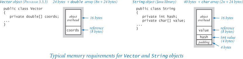
The class Vector (PROGRAM 3.3.3) includes an array as an instance variable. On a typical system, a Vector object of length n requires 8n + 48 bytes: the object overhead (16 bytes), a reference to a double array (8 bytes), and the memory for the double array (8n + 24 bytes). Thus, each of the Vector objects in Body uses 64 bytes of memory (since n = 2).

These basic mechanisms are effective for estimating the memory usage of a great many programs, but there are numerous complicating factors that can make the task significantly more difficult. We have already noted the potential effect of aliasing. Moreover, memory consumption is a complicated dynamic process when function calls are involved because the system memory allocation mechanism plays a more important role, with more system dependencies. For example, when your program calls a method, the system allocates the memory needed for the method (for its local variables) from a special area of memory called the stack; when the method returns to the caller, the memory is returned to the stack. For this reason, creating arrays or other large objects in recursive programs is dangerous, since each recursive call implies significant memory usage. When you create an object with new, the system allocates the memory needed for the object from another special area of memory known as the heap, and you must remember that every object lives until no references to it remain, at which point a system process known as garbage collection can reclaim its memory for the heap. Such dynamics can make the task of precisely estimating memory usage of a program challenging.

Perhaps the most common mistake made in programming is to pay too much attention to performance characteristics. Your first priority is to make your code clear and correct. Modifying a program for the sole purpose of speeding it up is best left for experts. Indeed, doing so is often counterproductive, as it tends to create code that is complicated and difficult to understand. C. A. R. Hoare (the inventor of quicksort and a leading proponent of writing clear and correct code) once summarized this idea by saying that “premature optimization is the root of all evil,” to which Knuth added the qualifier “(or at least most of it) in programming.” Beyond that, improving the running time is not worthwhile if the available cost benefits are insignificant. For example, improving the running time of a program by a factor of 10 is inconsequential if the running time is only an instant. Even when a program takes a few minutes to run, the total time required to implement and debug an improved algorithm might be substantially more than the time required simply to run a slightly slower one—you may as well let the computer do the work. Worse, you might spend a considerable amount of time and effort implementing ideas that should improve a program but actually do not do so.

Perhaps the second most common mistake made in developing an algorithm is to ignore performance characteristics. Faster algorithms are often more complicated than brute-force solutions, so you might be tempted to accept a slower algorithm to avoid having to deal with more complicated code. However, you can sometimes reap huge savings with just a few lines of good code. Users of a surprising number of computer systems lose substantial time waiting for simple quadratic-time algorithms to finish solving a problem, even though linear or linearithmic algorithms are available that are only slightly more complicated and could therefore solve the problem in a fraction of the time. When we are dealing with huge problem sizes, we often have no choice but to seek better algorithms.

Improving a program to make it clearer, more efficient, and elegant should be your goal every time that you work on it. If you pay attention to the cost all the way through the development of a program, you will reap the benefits every time you use it.

A. Run some experiments! The program TimePrimitives on the booksite uses Stopwatch to test the execution time of various arithmetic operations on primitive types. This technique measures the actual elapsed time as would be observed on a wall clock. If your system is not running many other applications, this can produce accurate results. You can find much more information about refining such experiments on the booksite.

Q. How much time does it take to call functions such as Math.sin(), Math.log(), and Math.sqrt() ?

A. Run some experiments! Stopwatch makes it easy to write programs such as TimePrimitives to answer questions of this sort for yourself, and you will be able to use your computer much more effectively if you get in the habit of doing so.

Q. How much time do string operations take?

A. Run some experiments! (Have you gotten the message yet?) A The String data type is implemented to allow the methods length() and charAt() to run in constant time. Methods such as toLowerCase() and replace() take time linear in the length of the string. The methods compareTo(), equals(), startsWith(), and endsWith() take time proportional to the number of characters needed to resolve the answer (constant time in the best case and linear time in the worst case), but indexOf() can be slow. String concatenation and the substring() method take time proportional to the total number of characters in the result.

Q. Why does allocating an array of length n take time proportional to n?

A. In Java, array elements are automatically initialized to default values (0, false, or null). In principle, this could be a constant-time operation if the system would defer initialization of each element until just before the program accesses that element for the first time, but most Java implementations go through the whole array to initialize each element.

Q. How do I determine how much memory is available for my Java programs?

A. Java will tell you when it runs out of memory, so it is not difficult to run some experiments. For example, if you use PrimeSieve (PROGRAM 1.4.3) by typing

% java PrimeSieve 100000000

and get the result

50847534

but then type

% java PrimeSieve 1000000000

and get the result

Click here to view code image

Exception in thread "main"
java.lang.OutOfMemoryError: Java heap space

then you can figure that you have enough room for a boolean array of length 100 million but not for a boolean array of length 1 billion. You can increase the amount of memory allotted to Java with command-line options. The following command executes PrimeSieve with the command-line argument 1000000000 and the command-line option -Xmx1110m, which requests a maximum of 1,100 megabytes of memory (if available).

Click here to view code image

% java -Xmx1100m PrimeSieve 1000000000

Q. What does it mean when someone says that the running time is O(n²)?

A. That is an example of a notation known as big-O notation. We write f(n) is O(g(n)) if there exist constants c and n₀ such that |f(n)| ≤ c |g(n)| for all n > n₀. In other words, the function f(n) is bounded above by g(n), up to constant factors and for sufficiently large values of n. For example, the function 30n² + 10n+ 7 is O(n²). We say that the worst-case running time of an algorithm is O(g(n)) if the running time as a function of the input size n is O(g(n)) for all possible inputs. Big-O notation and worst-case running times are widely used by theoretical computer scientists to prove theorems about algorithms, so you are sure to see this notation if you take a course in algorithms and data structures.

Q. So can I use the fact that the worst-case running time of an algorithm is O(n³) or O(n²) to predict performance?

A. Not necessarily, because the actual running time might be much less. For example, the function 30n² + 10n+ 7 is O(n²), but it is also O(n³) and O(n¹⁰) because big-O notation provides only an upper bound. Moreover, even if there is some family of inputs for which the running time is proportional to the given function, perhaps these inputs are not encountered in practice. Consequently, you should not use big-O notation to predict performance. The tilde notation and order-of-growth classifications that we use are more precise than big-O notation because they provide matching upper and lower bounds on the growth of the function. Many programmers incorrectly use big-O notation to indicate matching upper and lower bounds.

4.1.2 Modify ThreeSum to take an integer command-line argument target and find a triple of numbers on standard input whose sum is closest to target.

4.1.3 Write a program FourSum that reads long integers from standard input, and counts the number of 4-tuples that sum to zero. Use a quadruple nested loop. What is the order of growth of the running time of your program? Estimate the largest input size that your program can handle in an hour. Then, run your program to validate your hypothesis.

4.1.4 Prove by induction that the number of (unordered) pairs of integers between 0 and n–1 is n (n–1) / 2, and then prove by induction that the number of (unordered) triples of integers between 0 and n–1 is n (n–1)(n–2) / 6.

Answer for pairs: The formula is correct for n = 1, since there are 0 pairs. For n > 1, count all the pairs that do not include n–1, which is (n–1)(n–2) / 2 by the inductive hypothesis, and all the pairs that do include n–1, which is n–1, to get the total

(n–1)(n–2) / 2 +(n–1) = n (n–1) / 2

Answer for triples: The formula is correct for n = 2. For n > 2, count all the triples that do not include n–1, which is (n–1)(n–2)(n–3) / 6 by the inductive hypothesis, and all the triples that do include n–1, which is (n–1)(n–2) / 2, to get the total

(n–1)(n–2)(n–3) / 6 + (n–1)(n–2) / 2 = n (n–1)(n–2) / 6

4.1.5 Show by approximating with integrals that the number of distinct triples of integers between 0 and n is about n³/6.

Answer: Σ0nΣ0iΣ0j1≈∫0n∫0i∫0jdkdjdi=∫0n∫0ijdj⁢di=∫0n(i2/2)di=n3/6

4.1.6 Show that a log–log plot of the function cn^b has slope b and x-intercept log c. What are the slope and x-intercept for 4 n³ (log n)²?

4.1.7 What is the value of the variable count, as a function of n, after running the following code fragment?

Click here to view code image

long count = 0;
for (int i = 0; i < n; i++)
   for (int j = i + 1; j < n; j++)
      for (int k = j + 1; k < n; k++)
         count++;

Answer: n (n–1)(n–2) / 6

4.1.8 Use tilde notation to simplify each of the following formulas, and give the order of growth of each:

a. n (n – 1) (n – 2) (n – 3) / 24

b. (n – 2) (lg n – 2) (lg n + 2)

c. n (n +1) – n²

d. n (n +1) / 2 + n lg n

e. ln((n – 1)(n – 2) (n – 3))²

4.1.9 Determine the order of growth of the running time of this statement in ThreeSum as a function of the number of integers n on standard input:

Click here to view code image

int[] a = StdIn.readAllInts();

Answer: Linear. The bottlenecks are the implicit array initialization and the implicit input loop. Depending on your system, however, the cost of an input loop like this might dominate in a linearithmic-time or even a quadratic-time program unless the input size is sufficiently large.

4.1.10 Determine whether the following code fragment takes linear time, quadratic time, or cubic time (as a function of n).

Click here to view code image

for (int i = 0; i < n; i++)
   for (int j = 0; j < n; j++)
      if (i == j) c[i][j] = 1.0;
      else        c[i][j] = 0.0;

4.1.11 Suppose the running times of an algorithm for inputs of size 1,000, 2,000, 3,000, and 4,000 are 5 seconds, 20 seconds, 45 seconds, and 80 seconds, respectively. Estimate how long it will take to solve a problem of size 5,000. Is the algorithm linear, linearithmic, quadratic, cubic, or exponential?

4.1.12 Which would you prefer: an algorithm whose order of growth of running time is quadratic, linearithmic, or linear?

Answer: While it is tempting to make a quick decision based on the order of growth, it is very easy to be misled by doing so. You need to have some idea of the problem size and of the relative value of the leading coefficients of the running times. For example, suppose that the running times are n² seconds, 100 n log₂ n seconds, and 10,000 n seconds. The quadratic algorithm will be fastest for n up to about 1,000, and the linear algorithm will never be faster than the linearithmic one (n would have to be greater than 2¹⁰⁰, far too large to bother considering).

4.1.13 Apply the scientific method to develop and validate a hypothesis about the order of growth of the running time of the following code fragment, as a function of the argument n.

public static int f(int n)
{
   if (n == 0) return 1;
   return f(n-1) + f(n-1);
}

4.1.14 Apply the scientific method to develop and validate a hypothesis about the order of growth of the running time of the collect() method in Coupon (PROGRAM 2.1.3), as a function of the argument n. Note: Doubling is not effective for distinguishing between the linear and linearithmic hypotheses—you might try squaring the size of the input.

4.1.15 Apply the scientific method to develop and validate a hypothesis about the order of growth of the running time of Markov (PROGRAM 1.6.3), as a function of the command-line arguments trials and n.

4.1.16 Apply the scientific method to develop and validate a hypothesis about the order of growth of the running time of each of the following two code fragments as a function of n.

Click here to view code image

String s = "";
for (int i = 0; i < n; i++)
   if (StdRandom.bernoulli(0.5)) s += "0";
   else                          s += "1";

StringBuilder sb = new StringBuilder();
for (int i = 0; i < n; i++)
   if (StdRandom.bernoulli(0.5)) sb.append("0");
   else                          sb.append("1");
String s = sb.toString();

4.1.17 Each of the four Java functions given here returns a string of length n whose characters are all x. Determine the order of growth of the running time of each function. Recall that concatenating two strings in Java takes time proportional to the length of the resulting string.

Click here to view code image

public static String method1(int n)
{
   if (n == 0) return "";
   String temp = method1(n / 2);
   if (n % 2 == 0) return temp + temp;
   else            return temp + temp + "x";
}

public static String method2(int n)
{
   String s = "";
   for (int i = 0; i < n; i++)
      s = s + "x";
   return s;
}

Click here to view code image

public static String method3(int n)
{
   if (n == 0) return "";
   if (n == 1) return "x";
   return method3(n/2) + method3(n - n/2);
}

public static String method4(int n)
{
   char[] temp = new char[n];
   for (int i = 0; i < n; i++)
       temp[i] = 'x';
   return new String(temp);
}

4.1.18 The following code fragment (adapted from a Java programming book) creates a random permutation of the integers from 0 to n–1. Determine the order of growth of its running time as a function of n. Compare its order of growth with the shuffling code in SECTION 1.4.

Click here to view code image

int[] a = new int[n];
boolean[] taken = new boolean[n];
int count = 0;
while (count < n)
{
   int r = StdRandom.uniform(n);
   if (!taken[r])
   {
       a[r] = count;
       taken[r] = true;
       count++;
   }
}

4.1.19 What is the order of growth of the running time of the following two functions? Each function takes a string as an argument and returns the string reversed.

Click here to view code image

public static String reverse1(String s)
{
   int n = s.length();
   String reverse = "";
   for (int i = 0; i < n; i++)
      reverse = s.charAt(i) + reverse;
   return reverse;
}

public static String reverse2(String s)
{
   int n = s.length();
   if (n <= 1) return s;
   String left = s.substring(0, n/2);
   String right = s.substring(n/2, n);
   return reverse2(right) + reverse2(left);
}

4.1.20 Give a linear-time algorithm for reversing a string.

Answer:

Click here to view code image

public static String reverse(String s)
{
   int n = s.length();
   char[] a = new char[n];
   for (int i = 0; i < n; i++)
      a[i] = s.charAt(n-i-1);
   return new String(a);
}

4.1.21 Write a program MooresLaw that takes a command-line argument n and outputs the increase in processor speed over a decade if microprocessors double every n months. How much will processor speed increase over the next decade if speeds double every n = 15 months? 24 months?

4.1.22 Using the 64-bit memory model in the text, give the memory usage for an object of each of the following data types from CHAPTER 3:

a. Stopwatch

b. Turtle

c. Vector

d. Body

e. Universe

4.1.23 Estimate, as a function of the grid size n, the amount of space used by PercolationVisualizer (PROGRAM 2.4.3) with the vertical percolation detection (PROGRAM 2.4.2). Extra credit: Answer the same question for the case where the recursive percolation detection method (PROGRAM 2.4.5) is used.

4.1.24 Estimate the size of the biggest two-dimensional array of int values that your computer can hold, and then try to allocate such an array.

4.1.25 Estimate, as a function of the number of documents n and the dimension d, the amount of memory used by CompareDocuments (PROGRAM 3.3.5).

4.1.26 Write a version of PrimeSieve (PROGRAM 1.4.3) that uses a byte array instead of a boolean array and uses all the bits in each byte, thereby increasing the largest value of n that it can handle by a factor of 8.

4.1.27 The following table gives running times for three programs for various values of n. Fill in the blanks with estimates that you think are reasonable on the basis of the information given.

Give hypotheses for the order of growth of the running time of each program.

4.1.29 Closest pair. Design a quadratic-time algorithm that, given an array of integers, finds a pair that are closest to each other. (In the next section you will be asked to find a linearithmic algorithm for the problem.)

4.1.30 The “beck” exploit. A popular web server supports a function named no2slash() whose purpose is to collapse multiple / characters. For example, the string /d1///d2////d3/test.html collapses to /d1/d2/d3/test.html. The original algorithm was to repeatedly search for a / and copy the remainder of the string:

Click here to view code image

int n = name.length();
int i = 1;
while (i < n)
{
   if ((c[i-1] == '/') && (c[i] == '/'))
   {
      for(int j = i+1; j < n; j++)
         c[j-1] = c[j];
       n--;
   }
   else i++;
}

Unfortunately, this code can takes quadratic time (for example, if the string consists of the / character repeated n times). By sending multiple simultaneous requests with large numbers of / characters, a hacker could deluge the server and starve other processes for CPU time, thereby creating a denial-of-service attack. Develop a version of no2slash() that runs in linear time and does not allow for this type of attack.

4.1.31 Subset sum. Write a program SubsetSum that reads long integers from standard input, and counts the number of subsets of those integers that sum to exactly zero. Give the order of growth of the running time of your program.

4.1.32 Young tableaux. Suppose you have an n-by-n array of integers a[][] such that, for all i and j, a[i][j] < a[i+1][j] and a[i][j] < a[i][j+1], as in the following the 5-by-5 array.

 5  23  54  67  89
 6  69  73  74  90
10  71  83  84  91
60  73  84  86  92
89  91  92  93  94

A two-dimensional array with this property is known as a Young tableaux. Write a function that takes as arguments an n-by-n Young tableaux and an integer, and determines whether the integer is in the Young tableaux. The order of growth of the running time of your function should be linear in n.

4.1.33 Array rotation. Given an array of n elements, give a linear-time algorithm to rotate the string k positions. That is, if the array contains a₀, a₁, ..., a_n–1, the rotated array is a_k, a_k+1, ..., a_n-1, a₀, ..., a_k–1. Use at most a constant amount of extra memory. Hint: Reverse three subarrays.

4.1.34 Finding a repeated integer. (a) Given an array of n integers from 1 to n with one value repeated twice and one missing, give an algorithm that finds the missing integer, in linear time and constant extra memory. Integer overflow is not allowed. (b) Given a read-only array of n integers, where each value from 1 to n–1 occurs once and one occurs twice, give an algorithm that finds the duplicated value, in linear time and constant extra memory. (c) Given a read-only array of n integers with values between 1 and n–1, give an algorithm that finds a duplicated value, in linear time and constant extra memory.

4.1.35 Factorial. Design a fast algorithm to compute n! for large values of n, using Java’s BigInteger class. Use your program to compute the longest run of consecutive 9s in 1000000!. Develop and validate a hypothesis for the order of growth of the running time of your algorithm.

4.1.36 Maximum sum. Design a linear-time algorithm that finds a contiguous subarray of length at most m in an array of n long integers that has the highest sum among all such subarrays. Implement your algorithm, and confirm that the order of growth of its running time is linear.

4.1.37 Maximum average. Write a program that finds a contiguous subarray of length at most m in an array of n long integers that has the highest average value among all such subarrays, by trying all subarrays. Use the scientific method to confirm that the order of growth of the running time of your program is mn². Next, write a program that solves the problem by first computing the quantity prefix[i] = a[0] + ... + a[i] for each i, then computing the average in the interval from a[i] to a[j] with the expression (prefix[j] - prefix[i]) / (j - i + 1). Use the scientific method to confirm that this method reduces the order of growth by a factor of n.

4.1.38 Pattern matching. Given an n-by-n subarray of black (1) and white (0) pixels, design a linear-time algorithm that finds the largest square subarray that contains no white pixels. In the following example, the largest such subarray is the 3-by-3 subarray highlighted in blue.

1 0 1 1 1 0 0 0
0 0 0 1 0 1 0 0
0 0 1 1 1 0 0 0
0 0 1 1 1 0 1 0
0 0 1 1 1 1 1 1
0 1 0 1 1 1 1 0
0 1 0 1 1 0 1 0
0 0 0 1 1 1 1 0

Implement your algorithm and confirm that the order of growth of its running time is linear in the number of pixels. Extra credit: Design an algorithm to find the largest rectangular black subarray.

4.1.39 Sub-exponential function. Find a function whose order of growth is larger than any polynomial function, but smaller than any exponential function. Extra credit: Find a program whose running time has that order of growth.

Sorting and searching are important for commercial applications (businesses keep customer files in order) and scientific applications (to organize data and computation), and have all manner of applications in fields that may appear to have little to do with keeping things in order, including data compression, computer graphics, computational biology, numerical computing, combinatorial optimization, cryptography, and many others.

We use these fundamental problems to illustrate the idea that efficient algorithms are one key to effective solutions for computational problem. Indeed, many different sorting and searching methods have been proposed. Which should we use to address a given task? This question is important because different algorithms can have vastly differing performance characteristics, enough to make the difference between success in a practical situation and not coming close to doing so, even on the fastest available computer.

In this section, we will consider in detail two classical algorithms for sorting and searching—binary search and mergesort—along with several applications in which their efficiency plays a critical role. With these examples, you will be convinced not just of the utility of these methods, but also of the need to pay attention to the cost whenever you address a problem that requires a significant amount of computation.

As we discussed in SECTION 1.5, an effective strategy for the problem is to maintain an interval that contains the secret number. In each step, we ask a question that enables us to shrink the size of the interval in half. Specifically, we guess the number in the middle of the interval, and, depending on the answer, discard the half of the interval that cannot contain the secret number. More precisely, we use a half-open interval, which contains the left endpoint but not the right one. We use the notation [l o, hi) to denote all of the integers greater than or equal to lo and less than (but not equal to) hi. We start with lo = 0 and hi = n and use the following recursive strategy:

• Base case: If hi –lo equals 1, then the secret number is lo.

• Reduction step: Otherwise, ask whether the secret number is greater than or equal to the number mid = lo + (hi –lo)/2. If so, look for the number in [mid, hi); if not, look for the number in [lo, mid).

The function binarySearch() in Questions (PROGRAM 4.2.1) is an implementation of this strategy. It is an example of the general problem-solving technique known as binary search, which has many applications.

public class Questions
{
   public static int binarySearch(int lo, int hi)
   {  // Find number in [lo, hi)
      if (hi - lo == 1) return lo;
      int mid = lo + (hi - lo) / 2;
      StdOut.print("Greater than or equal to " + mid + "?  ");
      if (StdIn.readBoolean())
         return binarySearch(mid, hi);
      else
         return binarySearch(lo, mid);
   }

   public static void main(String[] args)
   {  // Play twenty questions.
      int k = Integer.parseInt(args[0]);
      int n = (int) Math.pow(2, k);
      StdOut.print("Think of a number ");
      StdOut.println("between 0 and " + (n-1));
      int guess = binarySearch(0, n);
      StdOut.println("Your number is " + guess);
   }
}

  lo   | smallest possible value
hi - 1 | largest possible value
  mid  | midpoint
   k   | number of questions
   n   | number of possible values

% java Questions 7
Think of a number between 0 and 127
Greater than or equal to 64?  false
Greater than or equal to 96?  true
Greater than or equal to 80?  true
Greater than or equal to 72?  false
Greater than or equal to 76?  false
Greater than or equal to 78?  true
Greater than or equal to 77?  false
Your number is 77

• The interval always contains the secret number.

• The interval sizes are the powers of 2, decreasing from n.

The first of these facts is enforced by the code; the second follows by noting that if (hi –lo) is a power of 2, then (hi –lo) / 2 is the next smaller power of 2 and also the size of both halved intervals [lo, mid) and [mid, hi). These facts are the basis of an induction proof that the algorithm operates as intended. Eventually, the interval size becomes 1, so we are guaranteed to find the number.

T(n) = T(n /2) + 1

with T(1) = 0. Substituting 2^k for n, we can telescope the recurrence (apply it to itself) to immediately get a closed-form expression:

T(2^k) = T(2^k–1) + 1 = T(2^k–2) + 2 = . . .= T(1) + k = k

Substituting back n for 2^k (and lg n for k) gives the result

T(n) = lg n

This justifies our hypothesis that the running time of binary search is logarithmic. Note: Binary search and TwentyQuestions.binarySearch() work even when n is not a power of 2—we assumed that n is a power of 2 to simplify our proof (see EXERCISE 4.2.1).

• Compute mid = lo + (hi –lo)/2.

• Base case: If hi –lo is less than δ, then return mid as an estimate of x.

• Reduction step: Otherwise, test whether f (mid) > y. If so, look for x in (lo, mid); if not, look for x in (mid, hi).

public static double inverseCDF(double y)
{  return bisectionSearch(y, 0.00000001, -8, 8);  }

private static double bisectionSearch(double y, double delta,
                                      double lo, double hi)
{  // Compute x with cdf(x) = y.
   double mid = lo + (hi - lo)/2;
   if (hi - lo < delta) return mid;
   if (cdf(mid) > y)
      return bisectionSearch(y, delta, lo, mid);
   else
      return bisectionSearch(y, delta, mid, hi);
}

  y   | argument
delta | desired precision
  lo  | smallest possible value
 mid  | midpoint
  hi  | largest possible value

To fix ideas, PROGRAM 4.2.2 computes the inverse of the Gaussian cumulative distribution function Φ, which we considered in Gaussian (PROGRAM 2.1.2).

The key to this method is the idea that the function is increasing—for any values a and b, knowing that f (a) < f (b) tells us that a < b, and vice versa. The recursive step just applies this knowledge: knowing that y = f (x) < f (mid) tells us that x < mid, so that x must be in the interval (lo, mid), and knowing that y = f (x) > f (mid) tells us that x > mid, so that x must be in the interval (mid, hi). You can think of the algorithm as determining which of the n = (hi–lo) / δ tiny intervals of size δ within (lo, hi) contains x, with running time logarithmic in n. As with number conversion for integers, we determine one bit of x for each iteration. In this context, binary search is often called bisection search because we bisect the interval at each stage.

public class BinarySearch
{
   public static int search(String key, String[] a)
   {  return search(key, a, 0, a.length);  }

   public static int search(String key, String[] a, int lo, int hi)
   {  // Search for key in a[lo, hi).
      if (hi <= lo) return -1;
      int mid = lo + (hi - lo) / 2;
      int cmp = a[mid].compareTo(key);
      if      (cmp > 0) return search(key, a, lo, mid);
      else if (cmp < 0) return search(key, a, mid+1, hi);
      else              return mid;
   }

   public static void main(String[] args)
   {  // Print keys from standard input that
      // do not appear in file args[0].
      In in = new In(args[0]);
      String[] a = in.readAllStrings();
      while (!StdIn.isEmpty())
      {
         String key = StdIn.readString();
         if (search(key, a) < 0) StdOut.println(key);
      }
   }
}

   key    | search key
a[lo, hi) | sorted subarray
   lo     | smallest index
  mid     | middle index
   hi     | largest index

% more emails.txt
bob@office
carl@beach
marvin@spam
bob@office
bob@office
mallory@spam
dave@boat
eve@airport
alice@home

% more whitelist.txt
alice@home
bob@office
carl@beach
dave@boat

% java BinarySearch whitelist.txt < emails.txt
marvin@spam
mallory@spam
eve@airport

The binary search in PROGRAM 4.2.3 differs from our other applications in two details. First, the array length n need not be a power of 2. Second, it has to allow for the possibility that the key sought is not in the array. Coding binary search to account for these details requires some care, as discussed in this section’s Q&A and exercises.

The test client in PROGRAM 4.2.3 is known as an exception filter: it reads in a sorted list of strings from a file (which we refer to as the whitelist) and an arbitrary sequence of strings from standard input, and prints those in the sequence that do not appear in the whitelist. Exception filters have many direct applications. For example, if the whitelist is the words from a dictionary and standard input is a text document, the exception filter prints the misspelled words. Another example arises in web applications: your email application might use an exception filter to reject any email messages that are not on a whitelist that contains the email addresses of your friends. Or, your operating system might have an exception filter that disallows network connections to your computer from any device having an IP address that is not on a preapproved whitelist.

Fast algorithms are an essential element of the modern world, and binary search is a prototypical example that illustrates the impact of fast algorithms. With a few quick calculations, you can convince yourself that problems like finding all the misspelled words in a document or protecting your computer from intruders using an exception filter require a fast algorithm like binary search. Take the time to do so. You can find the exceptions in a million-element document to a million-element whitelist in an instant, whereas that task might take days or weeks using a brute-force algorithm. Nowadays, web companies routinely provide services that are based on using binary search billions of times in sorted arrays with billions of elements—without a fast algorithm like binary search, we could not contemplate such services.

Whether it be extensive experimental data or detailed representations of some aspect of the physical world, modern scientists are awash in data. Binary search and fast algorithms like it are essential components of scientific progress. Using a brute-force algorithm is precisely analogous to searching for a word in a dictionary by starting at the first page and turning pages one by one. With a fast algorithm, you can search among billions of pieces of information in an instant. Taking the time to identify and use a fast algorithm for search certainly can make the difference between being able to solve a problem easily and spending substantial resources trying to do so (and failing).

The brute-force algorithm is known as insertion sort and is based on a simple method that people often use to arrange hands of playing cards. Consider the cards one at a time and insert each into its proper place among those already considered (keeping them sorted). The following code mimics this process in a Java method that rearranges the strings in an array so that they are in ascending order:

Click here to view code image

public static void sort(String[] a)
{
   int n = a.length;
   for (int i = 1; i < n; i++)
      for (int j = i; j > 0; j--)
         if (a[j-1].compareTo(a[j]) > 0)
              exchange(a, j-1, j);
         else break;
}

At the beginning of each iteration of the outer for loop, the first i elements in the array are in sorted order; the inner for loop moves a[i] into its proper position in the array, as in the following example when i is 6:

Specifically, a[i] is put in its place among the sorted elements to its left by exchanging it (using the exchange() method that we first encountered in SECTION 2.1) with each larger value to its left, moving from right to left, until it reaches its proper position. The black elements in the three bottom rows in this trace are the ones that are compared with a[i].

The insertion process just described is executed, first with i equal to 1, then 2, then 3, and so forth, as illustrated in the following trace.

Row i of the trace displays the contents of the array when the outer for loop completes, along with the value of j at that time. The highlighted string is the one that was in a[i] at the beginning of the loop, and the other strings printed in black are the other ones that were involved in exchanges and moved to the right one position within the loop. Since the elements a[0] through a[i-1] are in sorted order when the loop completes for each value of i, they are, in particular, in sorted order the final time the loop completes, when the value of i is a.length. This discussion again illustrates the first thing that you need to do when studying or developing a new algorithm: convince yourself that it is correct. Doing so provides the basic understanding that you need to study its performance and use it effectively.

A class that implements the Comparable interface promises to implement a method compareTo() for objects of its type so that a.compareTo(b) returns a negative integer (typically -1) if a is less than b, a positive integer (typically +1) if a is greater than b, and 0 if a is equal to b. (The <Key> notation, which we will introduce in SECTION 4.3, ensures that the two objects being compared have the same type.)

The precise meanings of less than, greater than, and equal to depends on the data type, though implementations that do not respect the natural laws of mathematics surrounding these concepts will yield unpredictable results. More formally, the compareTo() method must define a total order. This means that the following three properties must hold (where we use the notation x ≤ y as shorthand for x.compareTo(y) <= 0 and x = y as shorthand for x.compareTo(y) == 0):

• Antisymmetric: if both x ≤ y and y ≤ x, then x = y.

• Transitive: if both x ≤ y and y ≤ z, then x ≤ z.

• Total: either x ≤ y or y ≤ x or both.

These three properties hold for a variety of familiar orderings, including alphabetical order for strings and ascending order for integers and real numbers. We refer to a data type that implements the Comparable interface as comparable and the associated total order as its natural order. Java’s String type is comparable, as are the primitive wrapper types (such as Integer and Double) that we introduced in SECTION 3.3.

With this convention, Insertion (PROGRAM 4.2.4) implements our sort method so that it takes an array of comparable objects as an argument and rearranges the array so that its elements are in ascending order, according to the order specified by the compareTo() method. Now, we can use Insertion.sort() to sort arrays of type String[], Integer[], or Double[].

It is also easy to make a data type comparable, so that we can sort user-defined types of data. To do so, we must include the phrase implements Comparable in the class declaration, and then add a compareTo() method that defines a total order. For example, to make the Counter data type comparable, we modify PROGRAM 3.3.2 as follows:

Click here to view code image

public class Counter implements Comparable<Counter>
{
   private int count;
 ...
   public int compareTo(Counter b)
   {
     if      (count < b.count) return -1;
     else if (count > b.count) return +1;
     else                      return  0;
   }
 ...
}

Now, we can use Insertion.sort() to sort an array of Counter objects in ascending order of their counts.

public class Insertion
{
   public static void sort(Comparable[] a)
   {  // Sort a[] into increasing order.
      int n = a.length;
      for (int i = 1; i < n; i++)
         // Insert a[i] into position.
         for (int j = i; j > 0; j--)
            if (a[j].compareTo(a[j-1]) < 0)
                 exchange(a, j-1, j);
            else break;
   }

   public static void exchange(Comparable[] a, int i, int j)
   {  Comparable temp = a[j]; a[j] = a[i]; a[i] = temp;  }

   public static void main(String[] args)
   {  // Read strings from standard input, sort them, and print.
      String[] a = StdIn.readAllStrings();
      sort(a);
      for (int i = 0; i < a.length; i++)
         StdOut.print(a[i] + " ");
      StdOut.println();
   }
}

a[] | array to sort
 n  | length of array

The sort() function is an implementation of insertion sort. It sorts arrays of any type of data that implements the Comparable interface (and, therefore, has a compareTo() method). Insertion.sort() is appropriate only for small arrays or for arrays that are nearly in order; it is too slow to use for large arrays that are out of order.

% more 8words.txt
was had him and you his the but
% java Insertion < 8words.txt
and but had him his the was you
% java Insertion < TomSawyer.txt
tick tick tick tick tick tick tick tick tick tick tick tick tick tick tick tick tick tick tick tick
tick tick tick tick tick tick tick tick tick tick tick tick tick tick tick tick tick tick tick tick
tick tick tick tick tick tick tick tick tick tick tick tick tick tick tick tick tick tick tick tick
tick tick tick tick tick tick tick tick tick tick tick tick tick tick tick tick tick tick tick tick

There are many natural applications for which insertion sort is quadratic, so we need to consider faster sorting algorithms. As we know from SECTION 4.1, a back-ofthe-envelope calculation can tell us that having a faster computer is not much help. A dictionary, a scientific database, or a commercial database can contain billions of elements; how can we sort such a large array?

public class InsertionDoublingTest
{
   public static double timeTrials(int trials, int n)
   {  // Sort random arrays of size n.
      double total = 0.0;
      Double[] a = new Double[n];
      for (int t = 0; t < trials; t++)
      {
         for (int i = 0; i < n; i++)
            a[i] = StdRandom.uniform(0.0, 1.0);
         Stopwatch timer = new Stopwatch();
         Insertion.sort(a);
         total += timer.elapsedTime();
      }
      return total;
   }
   public static void main(String[] args)
   {  // Print doubling ratios for insertion sort.
      int trials = Integer.parseInt(args[0]);
      for (int n = 1024; true; n += n)
      {
         double prev = timeTrials(trials, n/2);
         double curr = timeTrials(trials, n);
         double ratio = curr / prev;
         StdOut.printf("%7d %4.2f
", n, ratio);
      }
   }
}

trials | number of trials
   n   | problem size
 total | total elapsed time
 timer | stopwatch
  a[]  | array to sort
 prev  | running time for n/2
 curr  | running time for n
 ratio | ratio of running times

% java InsertionDoublingTest 1
  1024 0.71
  2048 3.00
  4096 5.20
  8192 3.32
 16384 3.91
 32768 3.89

% java InsertionDoublingTest 10
  1024 1.89
  2048 5.00
  4096 3.58
  8192 4.09
 16384 4.83
 32768 3.96

We process contiguous subarrays of a given array, using the notation a[lo, hi) to refer to a[lo], a[lo+1], ..., a[hi-1] (adopting the same convention that we used for binary search to denote a half-open interval that excludes a[hi]). To sort a[lo, hi), we use the following recursive strategy:

• Base case: If the subarray length is 0 or 1, it is already sorted.

• Reduction step: Otherwise, compute mid = lo + (hi - lo)/2, recursively sort the two subarrays a[lo, mid) and a[mid, hi), and merge them.

Merge (PROGRAM 4.2.6) is an implementation of this algorithm. The values in the array are rearranged by the code that follows the recursive calls, which merges the two subarrays that were sorted by the recursive calls. As usual, the easiest way to understand the merge process is to study a trace during the merge. The code maintains one index i into the first subarray, another index j into the second subarray, and a third index k into an auxiliary array aux[] that temporarily holds the result. The merge implementation is a single loop that sets aux[k] to either a[i] or a[j] (and then increments k and the index the subarray that was used). If either i or j has reached the end of its subarray, aux[k] is set from the other; otherwise, it is set to the smaller of a[i] or a[j]. After all of the values from the two subarrays have been copied to aux[], the sorted result in aux[] is copied back to the original array. Take a moment to study the trace just given to convince yourself that this code always properly combines the two sorted subarrays to sort the full array.

The recursive method ensures that the two subarrays are each put into sorted order just prior to the merge. Again, the best way to gain an understanding of this process is to study a trace of the contents of the array each time the recursive sort() method returns. Such a trace for our example is shown next. First a[0] and a[1] are merged to make a sorted subarray in a[0, 2), then a[2] and a[3] are merged to make a sorted subarray in a[2, 4), then these two subarrays of size 2 are merged to make a sorted subarray in a[0, 4), and so forth. If you are convinced that the merge works properly, you need only convince yourself that the code properly divides the array to be convinced that the sort works properly. Note that when the number of elements in a subarray to be sorted is not even, the left half will have one fewer element than the right half.

sort(a, aux, 0, 8)
   sort(a, aux, 0, 4)
      sort(a, aux, 0, 2)
      return
      sort(a, aux, 2, 4)
      return
   return
   sort(a, aux, 4, 8)
      sort(a, aux, 4, 6)
      return
      sort(a, aux, 6, 8)
      return
   return
return

public class Merge

{
   public static void sort(Comparable[] a)
   {
      Comparable[] aux = new Comparable[a.length];
      sort(a, aux, 0, a.length);
   }

   private static void sort(Comparable[] a, Comparable[] aux,
                            int lo, int hi)
   {  // Sort a[lo, hi).
      if (hi - lo <= 1) return;
      int mid = lo + (hi-lo)/2;
      sort(a, aux, lo, mid);
      sort(a, aux, mid, hi);
      int i = lo, j = mid;
      for (int k = lo; k < hi; k++)
         if      (i == mid)  aux[k] = a[j++];
         else if (j == hi)   aux[k] = a[i++];
         else if (a[j].compareTo(a[i]) < 0) aux[k] = a[j++];
         else                               aux[k] = a[i++];
      for (int k = lo; k < hi; k++)
         a[k] = aux[k];
   }

   public static void main(String[] args)
   {  /* See Program 4.2.4. */  }
}

a[lo, hi) | subarray to sort
    lo    | smallest index
   mid    | middle index
    hi    | largest index
  aux[]   | auxiliary array

% java Merge < 8words.txt
was had him and you his the but

% java Merge < TomSawyer.txt
... achievement aching aching acquire acquired ...

You are encouraged to run a doubling test like PROGRAM 4.2.5 for Merge.sort() on your computer. If you do so, you certainly will appreciate that it is much faster for large arrays than is Insertion.sort() and that you can sort huge arrays with relative ease. Validating the hypothesis that the running time is linearithmic is a bit more work, but you certainly can see that mergesort makes it possible for us to address sorting problems that we could not contemplate solving with a brute-force algorithm such as insertion sort.

Mergesort traces back to John von Neumann, an accomplished physicist, who was among the first to recognize the importance of computation in scientific research. Von Neumann made many contributions to computer science, including a basic conception of the computer architecture that has been used since the 1950s. When it came to applications programming, von Neumann recognized that:

• Sorting is an essential ingredient in many applications.

• Quadratic-time algorithms are too slow for practical purposes.

• A divide-and-conquer approach is effective.

• Proving programs correct and knowing their cost is important.

Computers are many orders of magnitude faster and have many orders of magnitude more memory than those available to von Neumann, but these basic concepts remain important today. People who use computers effectively and successfully know, as did von Neumann, that brute-force algorithms are often not good enough to do the job.

to be or not to be to

then the result of the sort is

be be not or to to to

with equal strings—such as the two occurrences of be and the three occurrences of to—brought together in the array. Now, with equal strings all together in the array, we can make a single pass through the array to compute the frequencies. The Counter data type that we considered in SECTION 3.3 is the perfect tool for the job. Recall that a Counter (PROGRAM 3.3.2) has a string instance variable (initialized to the constructor argument), a count instance variable (initialized to 0), and an increment() instance method, which increments the counter by 1. We maintain an integer m and an array of Counter objects zipf[] and do the following for each string:

• If the string is not equal to the previous one, create a new Counter object and increment m.

• Increment the most recently created Counter.

At the end, the value of m is the number of different string values, and zipf[i] contains the ith string value and its frequency.

You are likely to find yourself writing a program sometime in the future for a simple task that could easily be solved by first using a sort. How many distinct values are there? Which value appears most frequently? What is the median value? With a linearithmic sorting algorithm such as mergesort, you can address these problems and many other problems like them, even for huge data sets. FrequencyCount, which uses two different sorts, is a prime example. If sorting does not apply directly, some other divide-and-conquer algorithm might apply, or some more sophisticated method might be needed. Without a good algorithm (and an understanding of its performance characteristics), you might find yourself frustrated by the idea that your fast and expensive computer cannot solve a problem that seems to be a simple one. With an ever-increasing set of problems that you know how to solve efficiently, you will find that your computer can be a much more effective tool than you now imagine.

---

Program 4.2.7 Frequency counts

Click here to view code image

public class FrequencyCount
{
   public static void main(String[] args)
   {  // Print input strings in decreasing order
      // of frequency of occurrence.
      String[] words = StdIn.readAllStrings();
      Merge.sort(words);
      Counter[] zipf = new Counter[words.length];
      int m = 0;
      for (int i = 0; i < words.length; i++)
      {  // Create new counter or increment prev counter.
         if (i == 0 || !words[i].equals(words[i-1]))
            zipf[m++] = new Counter(words[i], words.length);
         zipf[m-1].increment();
      }
      Merge.sort(zipf, 0, m);
      for (int j = m-1; j >= 0; j--)
         StdOut.println(zipf[j]);
    }
}

---

   s    | input
words[] | strings in input
zipf[]  | counter array
   m    | different strings

This program sorts the words on standard input, uses the sorted list to count the frequency of occurrence of each, and then sorts the frequencies. The test file used below has more than 20 million words. The plot compares the ith frequency relative to the first (bars) with 1/i (blue).

---

Click here to view code image

% java FrequencyCount < Leipzig1M.txt
the: 1160105
of: 593492
to: 560945
a: 472819
and: 435866
in: 430484
for: 205531
The: 192296
that: 188971
is: 172225
said: 148915
on: 147024
was: 141178
by: 118429
 ...

---

---

Since the advent of computing, people have been developing algorithms such as binary search and mergesort that can efficiently solve practical problems. The field of study known as design and analysis of algorithms encompasses the study of design paradigms such as divide-and-conquer and dynamic programming, the invention of algorithms for solving fundamental problems like sorting and searching, and techniques to develop hypotheses about the performance of algorithms. Implementations of many of these algorithms are found in Java libraries or other specialized libraries, but understanding these basic tools of computation is like understanding the basic tools of mathematics or science. You can use a matrix-processing package to find the eigenvalues of a matrix, but you still need a course in linear algebra. Now that you know a fast algorithm can make the difference between spinning your wheels and properly addressing a practical problem, you can be on the lookout for situations where algorithm design and analysis can make the difference, and where efficient algorithms such as binary search and mergesort can do the job.

A. To spare ourselves considerable pain. Binary search is a notable example. For example, you now understand binary search; a classic programming exercise is to write a version that uses a while loop instead of recursion. Try solving EXERCISE 4.2.2 without looking back at the code in the book. In a famous experiment, Jon Bentley once asked several professional programmers to do so, and most of their solutions were not correct.

Q. Are there implementations for sorting and searching in the Java library?

A. Yes. The Java package java.util contains the static methods Arrays.sort() and Arrays.binarySearch() that implement mergesort and binary search, respectively. Actually, each represents a family of overloaded methods, one for Comparable types, and one for each primitive type.

Q. So why not just use them?

A. Feel free to do so. As with many topics we have studied, you will be able to use such tools more effectively if you understand the background behind them.

Q. Explain why we use lo + (hi - lo) / 2 to compute the index midway between lo and hi instead of using (lo + hi) / 2.

A. The latter fails when lo + hi overflows an int.

Q. Why do I get a unchecked or unsafe operation warning when compiling Insertion.java and Merge.java?

A. The argument to sort() is a Comparable array, but nothing, technically, prevents its elements from being of different types. To eliminate the warning, change the signature to:

Click here to view code image

public static <Key extends Comparable<Key>> void sort(Key[] a)

We’ll learn about the <Key> notation in the next section when we discuss generics.

4.2.2 Develop a nonrecursive version of BinarySearch (PROGRAM 4.2.3).

4.2.3 Modify BinarySearch (PROGRAM 4.2.3) so that if the search key is in the array, it returns the smallest index i for which a[i] is equal to key, and otherwise returns -i, where i is the smallest index such that a[i] is greater than key.

4.2.4 Describe what happens if you apply binary search to an unordered array. Why shouldn’t you check whether the array is sorted before each call to binary search? Could you check that the elements binary search examines are in ascending order?

4.2.5 Describe why it is desirable to use immutable keys with binary search.

4.2.6 Add code to Insertion to produce the trace given in the text.

4.2.7 Add code to Merge to produce a trace like the following:

Click here to view code image

% java Merge < tiny.txt
was had him and you his the but
had was
        and him
and had him was
                his you
                        but the
                but his the you
and but had him his the was you

4.2.8 Give traces of insertion sort and mergesort in the style of the traces in the text, for the input it was the best of times it was.

4.2.9 Implement a more general version of PROGRAM 4.2.2 that applies bisection search to any monotonically increasing function. Use functional programming, in the same style as the numerical integration example from SECTION 3.3.

4.2.10 Write a filter DeDup that reads strings from standard input and prints them to standard output, with all duplicate strings removed (and in sorted order).

4.2.11 Modify StockAccount (PROGRAM 3.2.8) so that it implements the Comparable interface (comparing the stock accounts by name). Hint: Use the compareTo() method from the String data type for the heavy lifting.

4.2.12 Modify Vector (PROGRAM 3.3.3) so that it implements the Comparable interface (comparing the vectors lexicographically by coordinates).

4.2.13 Modify Time (EXERCISE 3.3.21) so that it implements the Comparable interface (comparing the times chronologically).

4.2.14 Modify Counter (PROGRAM 3.3.2) so that it implements the Comparable interface (comparing the objects by frequency count).

4.2.15 Add methods to Insertion (PROGRAM 4.2.4) and Merge (PROGRAM 4.2.6) to support sorting subarrays.

4.2.16 Develope a nonrecursive version of mergesort (PROGRAM 4.2.6). For simplicity, assume that the number of items n is a power of 2. Extra credit: Make your program work even if n is not a power of 2.

4.2.17 Find the frequency distribution of words in your favorite novel. Does it obey Zipf’s law?

4.2.18 Analyze mathematically the number of compares that mergesort makes to sort an array of length n. For simplicity, assume n is a power of 2.

Answer: Let M(n) be the number of compares to mergesort an array of length n. Merging two subarrays whose total length is n requires between ½ n and n–1 compares. Thus, M(n) satisfies the following recurrence relation:

M(n) ≤ 2M(n/2) + n

with M(1) = 0. Substituting 2^k for n gives

M(2^k) ≤ 2 M(2^k–1) + 2ⁿ

which is similar to, but more complicated than, the recurrence that we considered for binary search. But if we divide both sides by 2ⁿ, we get

M(2^k)/ 2^k ≤ M(2^k–1)/2^k–1 + 1

which is precisely the recurrence that we had for binary search. That is, M(2^k)/ 2^k ≤ T(2^k) = n. Substituting back n for 2^k (and lg n for k) gives the result M(n) ≤ n lg n. A similar argument shows that M(n) ≥ ½ n lg n.

4.2.19 Analyze mergesort for the case when n is not a power of 2.

Partial solution. When n is an odd number, one subarray has one more element than the other, so when n is not a power of 2, the subarrays on each level are not necessarily all the same size. Still, every element appears in some subarray, and the number of levels is still logarithmic, so the linearithmic hypothesis is justified for all n.

4.2.20 Median. Add to StdStats (PROGRAM 2.2.4) a method median() that computes in linearithmic time the median of an array of n integers. Hint: Reduce to sorting.

4.2.21 Mode. Add to StdStats (PROGRAM 2.2.4) a method mode() that computes in linearithmic time the mode (value that occurs most frequently) of an array of n integers. Hint: Reduce to sorting.

4.2.22 Integer sort. Write a linear-time filter that reads from standard input a sequence of integers that are between 0 and 99 and prints to standard output the same integers in sorted order. For example, presented with the input sequence

Click here to view code image

98 2 3 1 0 0 0 3 98 98 2 2 2 0 0 0 2

your program should print the output sequence

Click here to view code image

0 0 0 0 0 0 1 2 2 2 2 2 3 3 98 98 98

4.2.23 Floor and ceiling. Given a sorted array of Comparable items, write functions floor() and ceiling() that return the index of the largest (or smallest) item not larger (or smaller) than an argument item in logarithmic time.

4.2.24 Bitonic maximum. An array is bitonic if it consists of an increasing sequence of keys followed immediately by a decreasing sequence of keys. Given a bitonic array, design a logarithmic algorithm to find the index of a maximum key.

4.2.25 Search in a bitonic array. Given a bitonic array of n distinct integers, design a logarithmic-time algorithm to determine whether a given integer is in the array.

4.2.26 Closest pair. Given an array of n real numbers, design a linearithmic-time algorithm to find a pair of numbers that are closest in value.

4.2.27 Furthest pair. Given an array of n real numbers, design a linear-time algorithm to find a pair of numbers that are furthest apart in value.

4.2.28 Two sum. Given an array of n integers, design a linearithmic-time algorithm to determine whether any two of them sum to 0.

4.2.29 Three sum. Given an array of n integers, design an algorithm to determine whether any three of them sum to 0. The order of growth of the running time of your program should be n² log n. Extra credit: Develop a program that solves the problem in quadratic time.

4.2.30 Majority. A value in an array of length n is a majority if it appears strictly more than n / 2 times. Given an array of strings, design a linear-time algorithm to identify a majority element (if one exists).

4.2.31 Largest empty interval. Given n timestamps for when a file is requested from a web server, find the largest interval of time in which no file is requested. Write a program to solve this problem in linearithmic time.

4.2.32 Prefix-free codes. In data compression, a set of strings is prefix-free if no string is a prefix of another. For example, the set of strings { 01, 10, 0010, 1111 } is prefix-free, but the set of strings { 01, 10, 0010, 1010 } is not prefix-free because 10 is a prefix of 1010. Write a program that reads in a set of strings from standard input and determines whether the set is prefix-free.

4.2.33 Partitioning. Design a linear-time algorithm to sort an array of Comparable objects that is known to have at most two distinct values. Hint: Maintain two pointers, one starting at the left end and moving right, and the other starting at the right end and moving left. Maintain the invariant that all elements to the left of the left pointer are equal to the smaller of the two values and all elements to the right of the right pointer are equal to the larger of the two values.

4.2.34 Dutch-national-flag problem. Design a linear-time algorithm to sort an array of Comparable objects that is known to have at most three distinct values. (Edsger Dijkstra named this the Dutch-national-flag problem because the result is three “stripes” of values like the three stripes in the flag.)

4.2.35 Quicksort. Write a recursive program that sorts an array of Comparable objects by using, as a subroutine, the partitioning algorithm described in the previous exercise: First, pick a random element v as the partitioning element. Next, partition the array into a left subarray containing all elements less than v, followed by a middle subarray containing all elements equal to v, followed by a right subarray containing all elements greater than v. Finally, recursively sort the left and right subarrays.

4.2.36 Reverse domain name. Write a filter that reads a sequence of domain names from standard input and prints the reverse domain names in sorted order. For example, the reverse domain name of cs.princeton.edu is edu.princeton. cs. This computation is useful for web log analysis. To do so, create a data type Domain that implements the Comparable interface (using reverse-domain-name order).

4.2.37 Local minimum in an array. Given an array of n real numbers, design a logarithmic-time algorithm to identify a local minimum (an index i such that both a[i] < a[i-1] and a[i] < a[i+1]).

4.2.38 Discrete distribution. Design a fast algorithm to repeatedly generate numbers from the discrete distribution: Given an array a[] of non-negative real numbers that sum to 1, the goal is to return index i with probability a[i]. Form an array sum[] of cumulated sums such that sum[i] is the sum of the first i elements of a[]. Now, generate a random real number r between 0 and 1, and use binary search to return the index i for which sum[i] ≤ r < sum[i+1]. Compare the performance of this approach with the approach taken in RandomSurfer (PROGRAM 1.6.2).

4.2.39 Implied volatility. Typically the volatility σ is the unknown value in the Black–Scholes formula (see EXERCISE 2.1.28). Write a program that reads s, x, r, t, and the current price of the European call option from the command line and uses bisection search to compute σ.

4.2.40 Percolation threshold. Write a Percolation (PROGRAM 2.4.1) client that uses bisection search to estimate the percolation threshold value.