
A. If we changed a key while it was in the hash table or BST, it could invalidate the data structure’s invariants.
Q. Why is the val instance variable in the nested Node class in HashST declared to be of type Object instead of Value?
A. Good question. Unfortunately, as we saw in the Q&A at the end of SECTION 3.1, Java does not permit the creation of arrays of generics. One consequence of this restriction is that we need a cast in the get() method, which generates a compile-time warning (even though the cast is guaranteed to succeed at run time). Note that we can declare the val instance variable in the nested Node class in BST to be of type Value because it does not use arrays.
Q. Why not use the Java libraries for symbol tables?
A. Now that you understand how a symbol table works, you are certainly welcome to use the industrial-strength versions java.util.TreeMap and java.util.HashMap. They follow the same basic API as ST, but allow null keys and use the names containsKey() and keySet() instead of contains() and iterator(), respectively. They also contain a variety of additional utility methods, but they do not support some of the other methods that we mentioned, such as order statistics. You can also use java.util.TreeSet and java.util.HashSet, which implement an API like our SET.
Exercises
4.4.1 Modify Lookup to make a program LookupAndPut that allows put operations to be specified on standard input. Use the convention that a plus sign indicates that the next two strings typed are the key–value pair to be inserted.
4.4.2 Modify Lookup to make a program LookupMultiple that handles multiple values having the same key by storing all such values in a queue, as in Index, and then printing them all on a get request, as follows:
% java LookupMultiple amino.csv 3 0
Leucine
TTA TTG CTT CTC CTA CTG
4.4.3 Modify Index to make a program IndexByKeyword that takes a file name from the command line and makes an index from standard input using only the keywords in that file. Note: Using the same file for indexing and keywords should give the same result as Index.
4.4.4 Modify Index to make a program IndexLines that considers only consecutive sequences of letters as keys (no punctuation or numbers) and uses line number instead of word position as the value. This functionality is useful for programs, as follows:
% java IndexLines 6 0 < Index.java
continue 12
enqueue 15
Integer 4 5 7 8 14
parseInt 4 5
println 22
4.4.5 Develop an implementation BinarySearchST of the symbol-table API that maintains parallel arrays of keys and values, keeping them in key-sorted order. Use binary search for get, and move larger key–value pairs to the right one position for put (use a resizing array to keep the array length proportional to the number of key–value pairs in the table). Test your implementation with Index, and validate the hypothesis that using such an implementation for Index takes time proportional to the product of the number of strings and the number of distinct strings in the input.
4.4.6 Develop an implementation SequentialSearchST of the symbol-table API that maintains a linked list of nodes containing keys and values, keeping them in arbitrary order. Test your implementation with Index, and validate the hypothesis that using such an implementation for Index takes time proportional to the product of the number of strings and the number of distinct strings in the input.
4.4.7 Compute x.hashCode() % 5 for the single-character strings
E A S Y Q U E S T I O N
In the style of the drawing in the text, draw the hash table created when the ith key in this sequence is associated with the value i, for i from 0 to 11.
4.4.8 Implement the method contains() for HashST.
4.4.9 Implement the method size() for HashST.
4.4.10 Implement the method keys() for HashST.
4.4.11 Modify HashST to add a method remove() that takes a Key argument and removes that key (and the corresponding value) from the symbol table, if it exists.
4.4.12 Modify HashST to use a resizing array so that the average length of the list associated with each hash value is between 1 and 8.
4.4.13 Draw the BST that results when you insert the keys
E A S Y Q U E S T I O N
in that order into an initially empty tree. What is the height of the resulting BST?
4.4.14 Suppose we have integer keys between 1 and 1000 in a BST and search for 363. Which of the following cannot be the sequence of keys examined?
a. 2 252 401 398 330 363
b. 399 387 219 266 382 381 278 363
c. 3 923 220 911 244 898 258 362 363
d. 4 924 278 347 621 299 392 358 363
e. 5 925 202 910 245 363
4.4.15 Suppose that the following 31 keys appear (in some order) in a BST of height 4:
10 15 18 21 23 24 30 31 38 41 42 45 50 55 59
60 61 63 71 77 78 83 84 85 86 88 91 92 93 94 98
Draw the top three nodes of the tree (the root and its two children).
4.4.16 Draw all the different BSTs that can represent the sequence of keys
best of it the time was
4.4.17 True or false: Given a BST, let x be a leaf node, and let p be its parent. Then either (1) the key of p is the smallest key in the BST larger than the key of x or (2) the key of p is the largest key in the BST smaller than the key of x.
4.4.18 Implement the method contains() for BST.
4.4.19 Implement the method size() for BST.
4.4.20 Modify BST to add a method remove() that takes a Key argument and removes that key (and the corresponding value) from the symbol table, if it exists. Hint: Replace the key (and its associated value) with the next largest key in the BST (and its associated value); then remove from the BST the node that contained the next largest key.
4.4.21 Implement the method toString() for BST, using a recursive helper method like traverse(). As usual, you can accept quadratic performance because of the cost of string concatenation. Extra credit: Write a linear-time toString() method for BST that uses StringBuilder.
4.4.22 Modify the symbol-table API to handle values with duplicate keys by having get() return an iterable for the values having a given key. Implement BST and Index as dictated by this API. Discuss the pros and cons of this approach versus the one given in the text.
4.4.23 Modify BST to implement the SET API given at the end of this section.
4.4.24 Modify HashST to implement the SET API given at the end of this section (remover the Comparable restriction from the API).
4.4.25 A concordance is an alphabetical list of the words in a text that gives all word positions where each word appears. Thus, java Index 0 0 produces a concordance. In a famous incident, one group of researchers tried to establish credibility while keeping details of the Dead Sea Scrolls secret from others by making public a concordance. Write a program InvertConcordance that takes a command-line argument n, reads a concordance from standard input, and prints the first n words of the corresponding text on standard output.
4.4.26 Run experiments to validate the claims in the text that the put operations and get requests for Lookup and Index are logarithmic in the size of the table when using ST. Develop test clients that generate random keys and also run tests for various data sets, either from the booksite or of your own choosing.
4.4.27 Modify BST to add methods min() and max() that return the smallest (or largest) key in the table (or null if no such key exists).
4.4.28 Modify BST to add methods floor() and ceiling() that take as an argument a key and return the largest (smallest) key in the symbol table that is no larger (no smaller) than the specified key (or null if no such key exists).
4.4.29 Modify BST to add a method size() that returns the number of key–value pairs in the symbol table. Use the approach of storing within each Node the number of nodes in the subtree rooted there.
4.4.30 Modify BST to add a method rangeSearch() that takes two keys as arguments and returns an iterable over all keys that are between the two given keys. The running time should be proportional to the height of the tree plus the number of keys in the range.
4.4.31 Modify BST to add a method rangeCount() that takes two keys as arguments and returns the number of keys in a BST between the two specified keys. Your method should take time proportional to the height of the tree. Hint: First work the previous exercise.
4.4.32 Write an ST client that creates a symbol table mapping letter grades to numerical scores, as in the table below, and then reads from standard input a list of letter grades and computes their average (GPA).
 A+   A    A-   B+   B    B-   C+   C    C-   D    F
4.33 4.00 3.67 3.33 3.00 2.67 2.33 2.00 1.67 1.00 0.00
Binary Tree Exercises
These exercises are intended to give you experience in working with binary trees that are not necessarily BSTs. They all assume a Node class with three instance variables: a positive double value and two Node references. As with linked lists, you will find it helpful to make drawings using the visual representation shown in the text.
4.4.33 Implement the following methods, each of which takes as its argument a Node that is the root of a binary tree.
|
|
number of nodes in the tree |
|
|
number of nodes whose links are both |
|
|
sum of the key values in all nodes |
Your methods should all run in linear time.
4.4.34 Implement a linear-time method height() that returns the maximum number of links on any path from the root to a leaf node (the height of a one-node tree is 0).
4.4.35 A binary tree is heap ordered if the key at the root is larger than the keys in all of its descendants. Implement a linear-time method heapOrdered() that returns true if the tree is heap ordered, and false otherwise.
4.4.36 A binary tree is balanced if both its subtrees are balanced and the height of its two subtrees differ by at most 1. Implement a linear-time method balanced() that returns true if the tree is balanced, and false otherwise.
4.4.37 Two binary trees are isomorphic if only their key values differ (they have the same shape). Implement a linear-time static method isomorphic() that takes two tree references as arguments and returns true if they refer to isomorphic trees, and false otherwise. Then, implement a linear-time static method eq() that takes two tree references as arguments and returns true if they refer to identical trees (isomorphic with the same key values), and false otherwise.
4.4.38 Implement a linear-time method isBST() that returns true if the tree is a BST, and false otherwise.
Solution: This task is a bit more difficult than it might seem. Use an overloaded recursive method isBST() that takes two additional arguments lo and hi and returns true if the tree is a BST and all its values are between lo and hi, and use null to represent both the smallest possible and largest possible keys.
public static boolean isBST()
{  return isBST(root, null, null);  }

private boolean isBST(Node x, Key lo, Key hi)
{
   if (x == null) return true;
   if (lo != null && x.key.compareTo(lo) <= 0) return false;
   if (hi != null && x.key.compareTo(hi) >= 0) return false;
   if (!isBST(x.left, lo, x.key))   return false;
   if (!isBST(x.right, x.key, hi))  return false;
}
4.4.39 Write a method levelOrder() that prints BST keys in level order: first print the root; then the nodes one level below the root, left to right; then the nodes two levels below the root (left to right); and so forth. Hint: Use a Queue<Node>.
4.4.40 Compute the value returned by mystery() on some sample binary trees and then formulate a hypothesis about its behavior and prove it.
public int mystery(Node x)
{
   if (x == null) return 0;
   return mystery(x.left) + mystery(x.right);
}
Answer: Returns 0 for any binary tree.
Creative Exercises
4.4.41 Spell checking. Write a SET client SpellChecker that takes as a command-line argument the name of a file containing a dictionary of words, and then reads strings from standard input and prints any string that is not in the dictionary. You can find a dictionary file on the booksite. Extra credit: Augment your program to handle common suffixes such as -ing or -ed.
4.4.42 Spell correction. Write an ST client SpellCorrector that serves as a filter that replaces commonly misspelled words on standard input with a suggested replacement, printing the result to standard output. Take as a command-line argument the name of a file that contains common misspellings and corrections. You can find an example on the booksite.
4.4.43 Web filter. Write a SET client WebBlocker that takes as a command-line argument the name of a file containing a list of objectionable websites, and then reads strings from standard input and prints only those websites not on the list.
4.4.44 Set operations. Add methods union() and intersection() to SET that take two sets as arguments and return the union and intersection, respectively, of those two sets.
4.4.45 Frequency symbol table. Develop a data type FrequencyTable that supports the following operations: increment() and count(), both of which take string arguments. The data type keeps track of the number of times the increment() operation has been called with a given string as an argument. The increment() operation increments the count by 1, and the count() operation returns the count, possibly 0. Clients of this data type might include a web-traffic analyzer, a music player that counts the number of times each song has been played, phone software for counting calls, and so forth.
4.4.46 One-dimensional range searching. Develop a data type that supports the following operations: insert a date, search for a date, and count the number of dates in the data structure that lie in a particular interval. Use Java’s java.util.Date data type.
4.4.47 Non-overlapping interval search. Given a list of non-overlapping intervals of integers, write a function that takes an integer argument and determines in which, if any, interval that value lies. For example, if the intervals are 1643–2033, 5532–7643, 8999–10332, and 5666653–5669321, then the query point 9122 lies in the third interval and 8122 lies in no interval.
4.4.48 IP lookup by country. Write a BST client that uses the data file ip-to-country.csv found on the booksite to determine the source country of a given IP address. The data file has five fields: beginning of IP address range, end of IP address range, two-character country code, three-character country code, and country name. The IP addresses are non-overlapping. Such a database tool can be used for credit card fraud detection, spam filtering, auto-selection of language on a website, and web-server log analysis.
4.4.49 Inverted index of web. Given a list of web pages, create a symbol table of words contained in those web pages. Associate with each word a list of web pages in which that word appears. Write a program that reads in a list of web pages, creates the symbol table, and supports single-word queries by returning the list of web pages in which that query word appears.
4.4.50 Inverted index of web. Extend the previous exercise so that it supports multi-word queries. In this case, output the list of web pages that contain at least one occurrence of each of the query words.
4.4.51 Multiple word search. Write a program that takes k words from the command line, reads in a sequence of words from standard input, and identifies the smallest interval of text that contains all of the k words (not necessarily in the same order). You do not need to consider partial words.
Hint: For each index i, find the smallest interval [i, j] that contains the k query words. Keep a count of the number of times each of the k query words appears. Given [i, j], compute [i+1, j'] by decrementing the counter for word i. Then, gradually increase j until the interval contains at least one copy of each of the k words (or, equivalently, word i).
4.4.52 Repetition draw in chess. In the game of chess, if a board position is repeated three times with the same side to move, the side to move can declare a draw.
Describe how you could test this condition using a computer program.
4.4.53 Registrar scheduling. The registrar at a prominent northeastern university recently scheduled an instructor to teach two different classes at the same exact time. Help the registrar prevent future mistakes by describing a method to check for such conflicts. For simplicity, assume all classes run for 50 minutes and start at 9, 10, 11, 1, 2, or 3.
4.4.54 Random element. Add to BST a method random() that returns a random key. Maintain subtree sizes in each node (see EXERCISE 4.4.29). The running time should be proportional to the height of the tree.
4.4.55 Order statistics. Add to BST a method select() that takes an integer argument k and returns the kth smallest key in the BST. Maintain subtree sizes in each node (see EXERCISE 4.4.29). The running time should be proportional to the height of the tree.
4.4.56 Rank query. Add to BST a method rank() that takes a key as an argument and returns the number of keys in the BST that are strictly smaller than key. Maintain subtree sizes in each node (see EXERCISE 4.4.29). The running time should be proportional to the height of the tree.
4.4.57 Generalized queue. Implement a class that supports the following API, which generalizes both a queue and a stack by supporting removal of the ith least recently inserted item (see EXERCISE 4.3.40):
|
||
|
|
create an empty generalized queue |
|
|
is the generalized queue empty? |
|
|
insert |
|
|
remove and return the |
|
|
number of items in the queue |
API for a generic generalized queue |
||
Use a BST that associates the kth item inserted into the data structure with the key k and maintains in each node the total number of nodes in the subtree rooted at that node. To find the ith least recently inserted item, search for the ith smallest key in the BST.
4.4.58 Sparse vectors. A d-dimensional vector is sparse if its number of nonzero values is small. Your goal is to represent a vector with space proportional to its number of nonzeros, and to be able to add two sparse vectors in time proportional to the total number of nonzeros. Implement a class that supports the following API:
|
||
|
|
create a vector |
|
|
set ai to |
|
|
return ai |
|
|
vector dot product |
|
|
vector addition |
API for a sparse vector of |
||
4.4.59 Sparse matrices. An n-by-n matrix is sparse if its number of nonzeros is proportional to n (or less). Your goal is to represent a matrix with space proportional to n, and to be able to add and multiply two sparse matrices in time proportional to the total number of nonzeros (perhaps with an extra log n factor). Implement a class that supports the following API:
|
||
|
|
create a matrix |
|
|
set aij to |
|
|
return aij |
|
|
matrix addition |
|
|
matrix product |
API for a sparse matrix of |
||
4.4.60 Queue with no duplicates items. Create a data type that is a queue, except that an item may appear on the queue at most once at any given time. Ignore any request to insert an item if it is already on the queue.
4.4.61 Mutable string. Create a data type that supports the following API on a string. Use an ST to implement all operations in logarithmic time.
|
||
|
|
create an empty string |
|
|
return the |
|
|
insert |
|
|
delete the |
|
|
return the length of the string |
API for a mutable string |
||
4.4.62 Assignment statements. Write a program to parse and evaluate programs consisting of assignment and print statements with fully parenthesized arithmetic expressions (see PROGRAM 4.3.5). For example, given the input
A = 5
B = 10
C = A + B
D = C * C
print(D)
your program should print the value 225. Assume that all variables and values are of type double. Use a symbol table to keep track of variable names.
4.4.63 Entropy. We define the relative entropy of a text corpus with n words, k of which are distinct as
E = 1 / (n lg n) (p0 lg(k/p0) + p1 lg(k/p1) +... + pk–1 lg(k/pk–1))
where pi is the fraction of times that word i appears. Write a program that reads in a text corpus and prints the relative entropy. Convert all letters to lowercase and treat punctuation marks as whitespace.
4.4.64 Dynamic discrete distribution. Create a data type that supports the following two operations: add() and random(). The add() method should insert a new item into the data structure if it has not been seen before; otherwise, it should increase its frequency count by 1. The random() method should return an item at random, where the probabilities are weighted by the frequency of each item. Maintain subtree sizes in each node (see EXERCISE 4.4.29). The running time should be proportional to the height of the tree.
4.4.65 Stock account. Implement the two methods buy() and sell() in StockAccount (PROGRAM 3.2.8). Use a symbol table to store the number of shares of each stock.
4.4.66 Codon usage table. Write a program that uses a symbol table to print summary statistics for each codon in a genome taken from standard input (frequency per thousand), like the following:
UUU 13.2  UCU 19.6  UAU 16.5  UGU 12.4
UUC 23.5  UCC 10.6  UAC 14.7  UGC  8.0
UUA  5.8  UCA 16.1  UAA  0.7  UGA  0.3
UUG 17.6  UCG 11.8  UAG  0.2  UGG  9.5
CUU 21.2  CCU 10.4  CAU 13.3  CGU 10.5
CUC 13.5  CCC  4.9  CAC  8.2  CGC  4.2
CUA  6.5  CCA 41.0  CAA 24.9  CGA 10.7
CUG 10.7  CCG 10.1  CAG 11.4  CGG  3.7
AUU 27.1  ACU 25.6  AAU 27.2  AGU 11.9
AUC 23.3  ACC 13.3  AAC 21.0  AGC  6.8
AUA  5.9  ACA 17.1  AAA 32.7  AGA 14.2
AUG 22.3  ACG  9.2  AAG 23.9  AGG  2.8
GUU 25.7  GCU 24.2  GAU 49.4  GGU 11.8
GUC 15.3  GCC 12.6  GAC 22.1  GGC  7.0
GUA  8.7  GCA 16.8  GAA 39.8  GGA 47.2
4.4.67 Unique substrings of length k. Write a program that takes an integer command-line argument k, reads in text from standard input, and calculates the number of unique substrings of length k that it contains. For example, if the input is CGCCGGGCGCG, then there are five unique substrings of length 3: CGC, CGG, GCG, GGC, and GGG. This calculation is useful in data compression. Hint: Use the string method substring(i, i+k) to extract the ith substring and insert into a symbol table. Test your program on a large genome from the booksite and on the first 10 million digits of π.
4.4.68 Random phone numbers. Write a program that takes an integer command-line argument n and prints n random phone numbers of the form (xxx) xxx-xxxx. Use a SET to avoid choosing the same number more than once. Use only legal area codes (you can find a file of such codes on the booksite).
4.4.69 Password checker. Write a program that takes a string as a command-line argument, reads a dictionary of words from standard input, and checks whether the command-line argument is a “good” password. Here, assume “good” means that it (1) is at least eight characters long, (2) is not a word in the dictionary, (3) is not a word in the dictionary followed by a digit 0-9 (e.g., hello5), (4) is not two words separated by a digit (e.g., hello2world), and (5) none of (2) through (4) hold for reverses of words in the dictionary.
4.5 Case Study: Small-World Phenomenon
The mathematical model that we use for studying the nature of pairwise connections among entities is known as the graph. Graphs are important for studying the natural world and for helping us to better understand and refine the networks that we create. From models of the nervous system in neurobiology, to the study of the spread of infectious diseases in medical science, to the development of the telephone system, graphs have played a critical role in science and engineering over the past century, including the development of the Internet itself.
Some graphs exhibit a specific property known as the small-world phenomenon. You may be familiar with this property, which is sometimes known as six degrees of separation. It is the basic idea that, even though each of us has relatively few acquaintances, there is a relatively short chain of acquaintances (the six degrees of separation) separating us from one another. This hypothesis was validated experimentally by Stanley Milgram in the 1960s and modeled mathematically by Duncan Watts and Stephen Strogatz in the 1990s. In recent years, the principle has proved important in a remarkable variety of applications. Scientists are interested in small-world graphs because they model natural phenomena, and engineers are interested in building networks that take advantage of the natural properties of small-world graphs.
In this section, we address basic computational questions surrounding the study of small-world graphs. Indeed, the simple question
Does a given graph exhibit the small-world phenomenon?
can present a significant computational burden. To address this question, we will consider a graph-processing data type and several useful graph-processing clients. In particular, we will examine a client for computing shortest paths, a computation that has a vast number of important applications in its own right.
A persistent theme of this section is that the algorithms and data structures that we have been studying play a central role in graph processing. Indeed, you will see that several of the fundamental data types introduced earlier in this chapter help us to develop elegant and efficient code for studying the properties of graphs.
Graphs
To nip in the bud any terminological confusion, we start right away with some definitions. A graph comprises of a set of vertices and a set of edges. Each edge represents a connection between two vertices. Two vertices are adjacent if they are connected by an edge, and the degree of a vertex is its number of adjacent vertices (or neighbors). Note that there is no relationship between a graph and the idea of a function graph (a plot of a function values) or the idea of graphics (drawings). We often visualize graphs by drawing labeled circles (vertices) connected by lines (edges), but it is always important to remember that it is the connections that are essential, not the way we depict them.

The following list suggests the diverse range of systems where graphs are appropriate starting points for understanding structure.
Transportation systems
Train tracks connect stations, roads connect intersections, and airline routes connect airports, so all of these systems naturally admit a simple graph model. No doubt you have used applications that are based on such models when getting directions from an interactive mapping program or a GPS device, or when using an online service to make travel reservations. What is the best way to get from here to there?

system |
vertex |
edge |
natural phenomena |
||
circulatory |
organ |
blood vessel |
skeletal |
joint |
bone |
nervous |
neuron |
synapse |
social |
person |
relationship |
epidemiological |
person |
infection |
chemical |
molecule |
bond |
n-body |
particle |
force |
genetic |
gene |
mutation |
biochemical |
protein |
interaction |
engineered systems |
||
transportation |
airport |
route |
|
intersection |
road |
communication |
telephone |
wire |
|
computer |
cable |
|
web page |
link |
distribution |
power station home |
power line |
|
reservoir home |
pipe |
|
warehouse retail outlet |
truck route |
mechanical |
joint |
beam |
software |
module |
call |
financial |
account |
transaction |
Typical graph models |
||
Human biology
Arteries and veins connect organs, synapses connect neurons, and joints connect bones, so an understanding of the human biology depends on understanding appropriate graph models. Perhaps the largest and most important such modeling challenge in this arena is the human brain. How do local connections among neurons translate to consciousness, memory, and intelligence?
Social networks
People have relationships with other people. From the study of infectious diseases to the study of political trends, graph models of these relationships are critical to our understanding of their implications. Another fascinating problem is understanding how information propagates in online social networks.
Physical systems
Atoms connect to form molecules, molecules connect to form a material or a crystal, and particles are connected by mutual forces such as gravity or magnetism. For example, graph models are appropriate for studying the percolation problem that we considered in SECTION 2.4. How do local interactions propagate through such systems as they evolve?
Communications systems
From electric circuits, to the telephone system, to the Internet, to wireless services, communications systems are all based on the idea of connecting devices. For at least the past century, graph models have played a critical role in the development of such systems. What is the best way to connect the devices?
Resource distribution
Power lines connect power stations and home electrical systems, pipes connect reservoirs and home plumbing, and truck routes connect warehouses and retail outlets. The study of effective and reliable means of distributing resources depends on accurate graph models. Where are the bottlenecks in a distribution system?
Mechanical systems
Trusses or steel beams connect joints in a bridge or a building. Graph models help us to design these systems and to understand their properties. Which forces must a joint or a beam withstand?
Software systems
Methods in one program module invoke methods in other modules. As we have seen throughout this book, understanding relationships of this sort is a key to success in software design. Which modules will be affected by a change in an API?
Financial systems
Transactions connect accounts, and accounts connect customers to financial institutions. These are but a few of the graph models that people use to study complex financial transactions, and to profit from better understanding them. Which transactions are routine and which are indicative of a significant event that might translate into profits?

Some of these are models of natural phenomena, where our goal is to gain a better understanding of the natural world by developing simple models and then using them to formulate hypotheses that we can test. Other graph models are of networks that we engineer, where our goal is to design a better network or to better maintain a network by understanding its basic characteristics.
Graphs are useful models whether they are small or massive. A graph having just dozens of vertices and edges (for example, one modeling a chemical compound, where vertices are molecules and edges are bonds) is already a complicated combinatorial object because there are a huge number of possible graphs, so understanding the structures of the particular ones at hand is important. A graph having billions or trillions of vertices and edges (for example, a government database containing all phone-call metadata or a graph model of the human nervous system) is vastly more complex, and presents significant computational challenges.
Processing graphs typically involves building a graph from information in files and then answering questions about the graph. Beyond the application-specific questions in the examples just cited, we often need to ask basic questions about graphs. How many vertices and edges does the graph have? What are the neighbors of a given vertex? Some questions depend on an understanding of the structure of a graph. For example, a path in a graph is a sequence of adjacent vertices connected by edges. Is there a path connecting two given vertices? What is the length (number of edges) of the shortest path connecting two vertices? We have already seen in this book several examples of questions from scientific applications that are much more complicated than these. What is the probability that a random surfer will land on each vertex? What is the probability that a system represented by a certain graph percolates?

As you encounter complex systems in later courses, you are certain to encounter graphs in many different contexts. You may also study their properties in detail in later courses in mathematics, operations research, or computer science. Some graph-processing problems present insurmountable computational challenges; others can be solved with relative ease with data-type implementations of the sort we have been considering.
Graph data type
Graph-processing algorithms generally first build an internal representation of a graph by adding edges, then process it by iterating over the vertices and over the vertices adjacent to a given vertex. The following API supports such processing:
|
||
|
|
create an empty graph |
|
|
create graph from a file |
|
|
add edge |
|
|
number of vertices |
|
|
number of edges |
|
|
vertices in the graph |
|
|
neighbors of |
|
|
number of neighbors of |
|
|
is |
|
|
is |
API for a graph with |
||
As usual, this API reflects several design choices, each made from among various alternatives, some of which we now briefly discuss.
Undirected graph
Edges are undirected: an edge that connects v to w is the same as one that connects w to v. Our interest is in the connection, not the direction. Directed edges (for example, one-way streets in road maps) require a slightly different data type (see EXERCISE 4.5.41).
String vertex type
We might use a generic vertex type, to allow clients to build graphs with objects of any type. We leave this sort of implementation for an exercise, however, because the resulting code becomes a bit unwieldy (see EXERCISE 4.5.9). The String vertex type suffices for the applications that we consider here.
Invalid vertex names
The methods adjacentTo(), degree(), and hasEdge() all throw an exception if called with a string argument that does not correspond to a vertex name. The client can call hasVertex() to detect such situations.
Implicit vertex creation
When a string is used as an argument to addEdge(), we assume that it is a vertex name. If no vertex using that name has yet been added, our implementation adds such a vertex. The alternative design of having an addVertex() method requires more client code (to create the vertices) and more cumbersome implementation code (to check that edges connect vertices that have previously been created).
Self-loops and parallel edges
Although the API does not explicitly address the issue, we assume that implementations do allow self-loops (edges connecting a vertex to itself) but do not allow parallel edges (two copies of the same edge). Checking for self-loops and parallel edges is easy; our choice is to omit both checks.
Client query methods
We also include the methods V() and E() in our API to provide to the client the number of vertices and edges in the graph. Similarly, the methods degree(), hasVertex(), and hasEdge() are useful in client code. We leave the implementation of these methods as exercises, but assume them to be in our Graph API.
None of these design decisions are sacrosanct; they are simply the choices that we have made for the code in this book. Some other choices might be appropriate in various situations, and some decisions are still left to implementations. It is wise to carefully consider the choices that you make for design decisions like this and to be prepared to defend them.
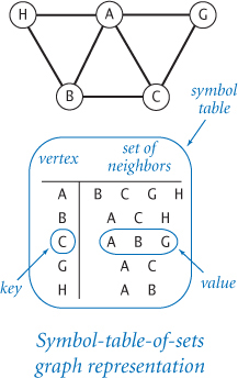
Graph (PROGRAM 4.5.1) implements this API. Its internal representation is a symbol table of sets: the keys are vertices and the values are the sets of neighbors—the vertices adjacent to the key. This representation uses the two data types ST and SET that we introduced in SECTION 4.4. It has three important properties:
• Clients can efficiently iterate over the graph vertices.
• Clients can efficiently iterate over a vertex’s neighbors.
• Memory usage is proportional to the number of edges.
These properties follow immediately from basic properties of ST and SET. As you will see, these two iterators are at the heart of graph processing.
public class Graph
{
   private ST<String, SET<String>> st;

   public Graph()
   {  st = new ST<String, SET<String>>();  }

   public void addEdge(String v, String w)
   {  // Put v in w's SET and w in v's SET.
      if (!st.contains(v)) st.put(v, new SET<String>());
      if (!st.contains(w)) st.put(w, new SET<String>());
      st.get(v).add(w);
      st.get(w).add(v);
   }

   public Iterable<String> adjacentTo(String v)
   {  return st.get(v);  }

   public Iterable<String> vertices()
   {  return st.keys();  }

   // See Exercises 4.5.1-4 for V(), E(), degree(),
   // hasVertex(), and hasEdge().

   public static void main(String[] args)
   {  // Read edges from standard input; print resulting graph.
      Graph G = new Graph();
      while (!StdIn.isEmpty())
         G.addEdge(StdIn.readString(), StdIn.readString());
      StdOut.print(G);
   }
}
st | symbol table of vertex neighbor sets
This implementation uses ST and SET (see SECTION 4.4) to implement the graph data type. Clients build graphs by adding edges and process them by iterating over the vertices and then over the set of vertices adjacent to each vertex. See the text for toString() and a matching constructor that reads a graph from a file.
% more tinyGraph.txt
A B
A C
C G
A G
H A
B C
B H
% java Graph < tinyGraph.txt
A  B C G H
B  A C H
C  A B G
G  A C
H  A B
As a simple example of client code, consider the problem of printing a Graph. A natural way to proceed is to print a list of the vertices, along with a list of the neighbors of each vertex. We use this approach to implement toString() in Graph, as follows:
public String toString()
{
   String s = "";
   for (String v : vertices())
   {
      s += v + "  ";
      for (String w : adjacentTo(v))
         s += w + " ";
      s += "
";
   }
   return s;
}
This code prints two representations of each edge—once when discovering that w is a neighbor of v, and once when discovering that v is a neighbor of w. Many graph algorithms are based on this basic paradigm of processing each edge in the graph in this way, and it is important to remember that they process each edge twice. As usual, this implementation is intended for use only for small graphs, as the running time is quadratic in the string length because string concatenation is linear time.
The output format just considered defines a reasonable file format: each line is a vertex name followed by the names of neighbors of that vertex. Accordingly, our basic graph API includes a constructor for building a graph from a file in this format (list of vertices with neighbors). For flexibility, we allow for the use of other delimiters besides spaces for vertex names (so that, for example, vertex names may contain spaces), as in the following implementation:
public Graph(String filename, String delimiter)
{
   st = new ST<String, SET<String>>();
   In in = new In(filename);
   while (in.hasNextLine())
   {
      String line = in.readLine();
      String[] names = line.split(delimiter);
      for (int i = 1; i < names.length; i++)
         addEdge(names[0], names[i]);
   }
}
Adding this constructor and toString() to Graph provides a complete data type suitable for a broad variety of applications, as we will now see. Note that this same constructor (with a space delimiter) works properly when the input is a list of edges, one per line, as in the test client for PROGRAM 4.5.1.
Graph client example
As a first graph-processing client, we consider an example of social relationships, one that is certainly familiar to you and for which extensive data is readily available.
On the booksite you can find the file movies.txt (and many similar files), which contains a list of movies and the performers who appeared in them. Each line gives the name of a movie followed by the cast (a list of the names of the performers who appeared in that movie). Since names have spaces and commas in them, the / character is used as a delimiter. (Now you can see why our second Graph constructor takes the delimiter as an argument.)
If you study movies.txt, you will notice a number of characteristics that, though minor, need attention when working with the database:
• Movies always have the year in parentheses after the title.
• Special characters are present.
• Multiple performers with the same name are differentiated by Roman numerals within parentheses.
• Cast lists are not in alphabetical order.
Depending on your terminal window and operating system settings, special characters may be replaced by blanks or question marks. These types of anomalies are common when working with large amounts of real-world data. You can either choose to live with them or configure your environment properly (see the booksite for details).
% more movies.txt
...
Tin Men (1987)/DeBoy, David/Blumenfeld, Alan/... /Geppi, Cindy/Hershey, Barbara
Tirez sur le pianiste (1960)/Heymann, Claude/.../Berger, Nicole (I)
Titanic (1997)/Mazin, Stan/...DiCaprio, Leonardo/.../Winslet, Kate/...
Titus (1999)/Weisskopf, Hermann/Rhys, Matthew/.../McEwan, Geraldine
To Be or Not to Be (1942)/Verebes, Ernö (I)/.../Lombard, Carole (I)
To Be or Not to Be (1983)/.../Brooks, Mel (I)/.../Bancroft, Anne/...
To Catch a Thief (1955)/París, Manuel/.../Grant, Cary/.../Kelly, Grace/...
To Die For (1995)/Smith, Kurtwood/.../Kidman, Nicole/.../ Tucci, Maria
...
Movie database example

Using Graph, we can write a simple and convenient client for extracting information from the file movies.txt. We begin by building a Graph to better structure the information. What should the vertices and edges model? Should the vertices be movies with edges connecting two movies if a performer has appeared in both? Should the vertices be performers with edges connecting two performers if both have appeared in the same movie? Both choices are plausible, but which should we use? This decision affects both client and implementation code. Another way to proceed (which we choose because it leads to simple implementation code) is to have vertices for both the movies and the performers, with an edge connecting each movie to each performer in that movie. As you will see, programs that process this graph can answer a great variety of interesting questions. IndexGraph (PROGRAM 4.5.2) is a first example that takes a query, such as the name of a movie, and prints the list of performers who appear in that movie.
Program 4.5.2 Using a graph to invert an index
public class IndexGraph
{
   public static void main(String[] args)
   {  // Build a graph and process queries.
      String filename = args[0];
      String delimiter = args[1];
      Graph G = new Graph(filename, delimiter);
      while (StdIn.hasNextLine())
      {  // Read a vertex and print its neighbors.
         String v = StdIn.readLine();
         for (String w : G.adjacentTo(v))
            StdOut.println("  " + w);
      }
   }
}
    filename    | filename
delimiter | input delimiter
    G     | graph
    v     | query
    w     | neighbor of v
This Graph client creates a graph from the file specified on the command line, then reads vertex names from standard input and prints its neighbors. When the file corresponds to a movie–cast list, the graph is bipartite and this program amounts to an interactive inverted index.
% java IndexGraph movies.txt "/"
Da Vinci Code, The (2006)
  Aubert, Yves
  ...
  Herbert, Paul
  ...
  Wilson, Serretta
  Zaza, Shane
Bacon, Kevin
  Animal House (1978)
  Apollo 13 (1995)
  ...
  Wild Things (1998)
  River Wild, The (1994)
  Woodsman, The (2004)
Typing a movie name and getting its cast is not much more than regurgitating the corresponding line in movies.txt (though IndexGraph prints the cast list sorted by last name, as that is the default iteration order provided by SET). A more interesting feature of IndexGraph is that you can type the name of a performer and get the list of movies in which that performer has appeared. Why does this work? Even though movies.txt seems to connect movies to performers and not the other way around, the edges in the graph are connections that also connect performers to movies.
A graph in which connections all connect one kind of vertex to another kind of vertex is known as a bipartite graph. As this example illustrates, bipartite graphs have many natural properties that we can often exploit in interesting ways.
As we saw at the beginning of SECTION 4.4, the indexing paradigm is general and very familiar. It is worth reflecting on the fact that building a bipartite graph provides a simple way to automatically invert any index! The file movies.txt is indexed by movie, but we can query it by performer. You could use IndexGraph in precisely the same way to print the index words appearing on a given page or the codons corresponding to a given amino acid, or to invert any of the other indices discussed at the beginning of SECTION 4.2. Since IndexGraph takes the delimiter as a command-line argument, you can use it to create an interactive inverted index for a .csv.
% more amino.csv
TTT,Phe,F,Phenylalanine
TTC,Phe,F,Phenylalanine
TTA,Leu,L,Leucine
TTG,Leu,L,Leucine
TCT,Ser,S,Serine
TCC,Ser,S,Serine
TCA,Ser,S,Serine
TCG,Ser,S,Serine
TAT,Tyr,Y,Tyrosine
...
GGA,Gly,G,Glycine
GGG,Gly,G,Glycine

% java IndexGraph amino.csv ","
TTA
  Lue
  L
  Leucine
Serine
  TCT
  TCC
  TCA
  TCG
Inverting an index
This inverted-index functionality is a direct benefit of the graph data structure. Next, we examine some of the added benefits to be derived from algorithms that process the data structure.
Shortest paths in graphs
Given two vertices in a graph, a path is a sequence of edges connecting them. A shortest path is one with the minimal length or distance (number of edges) over all such paths (there typically are multiple shortest paths). Finding a shortest path connecting two vertices in a graph is a fundamental problem in computer science. Shortest paths have been famously and successfully applied to solve large-scale problems in a broad variety of applications, from Internet routing to financial transactions to the dynamics of neurons in the brain.
As an example, imagine that you are a customer of an imaginary no-frills airline that serves a limited number of cities with a limited number of routes. Assume that the best way to get from one place to another is to minimize your number of flight segments, because delays in transferring from one flight to another are likely to be lengthy. A shortest-path algorithm is just what you need to plan a trip. Such an application appeals to our intuition in understanding the basic problem and our approach to solving it. After covering these topics in the context of this example, we will consider an application where the graph model is more abstract.
Depending upon the application, clients have various needs with regard to shortest paths. Do we want the shortest path connecting two given vertices? Or just the length of such a path? Will we have a large number of such queries? Is one particular vertex of special interest? In huge graphs or for huge numbers of queries, we have to pay particular attention to such questions because the cost of computing shortest paths might prove to be prohibitive. We start with the following API:
|
||
|
|
constructor |
|
|
length of shortest path from |
|
|
shortest path from |
API for single-source shortest paths in a |
||
Clients can construct a PathFinder object for a given graph G and source vertex s, and then use that object either to find the length of a shortest path or to iterate over the vertices on a shortest path from s to any other vertex in G. An implementation of these methods is known as a single-source shortest-path algorithm. We will consider a classic algorithm for the problem, known as breadth-first search, which provides a direct and elegant solution.
Single-source client
Suppose that you have available to you the graph of vertices and connections for your no-frills airline’s route map. Then, using your home city as the source, you can write a client that prints your route anytime you want to go on a trip. PROGRAM 4.5.3 is a client for PathFinder that provides this functionality for any graph. This sort of client is particularly useful in applications where we anticipate numerous queries from the same source. In this situation, the cost of building a PathFinder object is amortized over the cost of all the queries. You are encouraged to explore the properties of shortest paths by running PathFinder on our sample input file routes.txt.

Degrees of separation
One of the classic applications of shortest-paths algorithms is to find the degrees of separation of individuals in social networks. To fix ideas, we discuss this application in terms of a popular pastime known as the Kevin Bacon game, which uses the movie–performer graph that we just considered. Kevin Bacon is a prolific actor who has appeared in many movies. We assign every performer who has appeared in a movie a Kevin Bacon number: Bacon himself is 0, any performer who has been in the same cast as Bacon has a Kevin Bacon number of 1, any other performer (except Bacon) who has been in the same cast as a performer whose number is 1 has a Kevin Bacon number of 2, and so forth. For example, Meryl Streep has a Kevin Bacon number of 1 because she appeared in The River Wild with Kevin Bacon. Nicole Kidman’s number is 2: although she did not appear in any movie with Kevin Bacon, she was in Cold Mountain with Donald Sutherland, and Sutherland appeared in Animal House with Kevin Bacon. Given the name of a performer, the simplest version of the game is to find some alternating sequence of movies and performers that leads back to Kevin Bacon. For example, a movie buff might know that Tom Hanks was in Joe Versus the Volcano with Lloyd Bridges, who was in High Noon with Grace Kelly, who was in Dial M for Murder with Patrick Allen, who was in The Eagle Has Landed with Donald Sutherland, who we know was in Animal House with Kevin Bacon. But this knowledge does not suffice to establish Tom Hanks’s Bacon number (it is actually 1 because he was in Apollo 13 with Kevin Bacon). You can see that the Kevin Bacon number has to be defined by counting the movies in the shortest such sequence, so it is hard to be sure whether someone wins the game without using a computer. Remarkably, the PathFinder test client in PROGRAM 4.5.3 is just the program you need to find a shortest path that establishes the Kevin Bacon number of any performer in movies.txt—the number is precisely half the distance. You might enjoy using this program, or extending it to answer some entertaining questions about the movie business or in one of many other domains. For example, mathematicians play this same game with the graph defined by paper co-authorship and their connection to Paul Erdös, a prolific 20th-century mathematician. Similarly, everyone in New Jersey seems to have a Bruce Springsteen number of 2, because everyone in the state seems to know someone who claims to know Bruce.
Program 4.5.3 Shortest-paths client
public class PathFinder
{
   // See Program 4.5.4 for implementation.

   public static void main(String[] args)
   {
      // Read graph and compute shortest paths from s.
      String filename = args[0];
      String delimiter = args[1];
      Graph G = new Graph(filename, delimiter);
      String s = args[2];
      PathFinder pf = new PathFinder(G, s);

      // Process queries.
      while (StdIn.hasNextLine())
      {
         String t = StdIn.readLine();
         int d = pf.distanceTo(t);
         for (String v : pf.pathTo(t))
            StdOut.println("   " + v);
         StdOut.println("distance " + d);
      }
   }
}
 filename | filename
delimiter | input delimiter
    G     | graph
    s     | source
    pf    | PathFinder from s
    t     | destination query
    v     | vertex on path
This PathFinder client takes the name of a file, a delimiter, and a source vertex as command-line arguments. It builds a graph from the file, assuming that each line of the file specifies a vertex and a list of vertices connected to that vertex, separated by the delimiter. When you type a destination on standard input, you get the shortest path from the source to that destination.
% more routes.txt
JFK MCO
ORD DEN
PHX LAX
ORD HOU
DFW PHX
ORD DFW
...
JFK ORD
HOU MCO
LAS PHX
% java PathFinder routes.txt " " JFK
LAX
    JFK
    ORD
    PHX
    LAX
distance 3
DFW
    JFK
    ORD
    DFW
distance 2
% java PathFinder movies.txt "/" "Bacon, Kevin"
Kidman, Nicole
   Bacon, Kevin
   Animal House (1978)
   Sutherland, Donald (I)
   Cold Mountain (2003)
   Kidman, Nicole
distance 4
Hanks, Tom
   Bacon, Kevin
   Apollo 13 (1995)
   Hanks, Tom
distance 2
Degrees of separation from Kevin Bacon
Other clients
PathFinder is a versatile data type that can be put to many practical uses. For example, it is easy to develop a client that handles arbitrary source-destination requests on standard input, by building a PathFinder for each vertex (see EXERCISE 4.5.17). Travel services use precisely this approach to handle requests at a very high service rate. Since this client builds a PathFinder for each vertex (each of which might consume memory proportional to the number of vertices), memory usage might be a limiting factor in using it for huge graphs. For an even more performance-critical application that is conceptually the same, consider an Internet router that has a graph of connections among machines available and must decide the best next stop for packets heading to a given destination. To do so, it can build a PathFinder with itself as the source; then, to send a packet to destination w, it computes pf.pathTo(w) and sends the packet to the first vertex on that path—the next stop on the shortest path to w. Or a central authority might build a PathFinder object for each of several dependent routers and use them to issue routing instructions. The ability to handle such requests at a high service rate is one of the prime responsibilities of Internet routers, and shortest-paths algorithms are a critical part of the process.
Shortest-path distances
The first step in understanding breadth-first search is to consider the problem of computing the lengths of the shortest paths from the source to each other vertex. Our approach is to compute and save away all the distances in the PathFinder constructor, and then just return the requested value when a client invokes distanceTo(). To associate an integer distance with each vertex name, we use a symbol table:
ST<String, Integer> dist = new ST<String, Integer>();

The purpose of this symbol table is to associate with each vertex an integer: the length of the shortest path (the distance) from s to that vertex. We begin by associating the distance 0 with s via the call dist.put(s, 0), and we associate the distance 1 with s’s neighbors using the following code:
for (String v : G.adjacentTo(s))
   dist.put(v, 1)
But then what do we do? If we blindly set the distances to all the neighbors of each of those neighbors to 2, then not only would we face the prospect of unnecessarily setting many values twice (neighbors may have many common neighbors), but also we would set s’s distance to 2 (it is a neighbor of each of its neighbors), and we clearly do not want that outcome. The solution to these difficulties is simple:
• Consider the vertices in order of their distance from s.
• Ignore vertices whose distance to s is already known.
To organize the computation, we use a FIFO queue. Starting with s on the queue, we perform the following operations until the queue is empty:
• Dequeue a vertex v.
• Assign all of v’s unknown neighbors a distance 1 greater than v’s distance.
• Enqueue all of the unknown neighbors.
Breadth-first search dequeues the vertices in nondecreasing order of their distance from the source s. Tracing this algorithm on a sample graph will help to persuade you that it is correct. Showing that breadth-first search labels each vertex v with its distance to s is an exercise in mathematical induction (see EXERCISE 4.5.12).
Shortest-paths tree
We want not only the lengths of the shortest paths, but also the shortest paths themselves. To implement pathTo(), we use a subgraph known as the shortest-paths tree, defined as follows:
• Put the source at the root of the tree.
• Put vertex v’s neighbors in the tree if they are added to the queue when processing vertex v, with an edge connecting each to v.
Since we enqueue each vertex only once, this structure is a proper tree: it consists of a root (the source) connected to one subtree for each neighbor of the source. Studying such a tree, you can see immediately that the distance from each vertex to the root in the tree is the same as the length of the shortest path from the source in the graph. More importantly, each path in the tree is a shortest path in the graph. This observation is important because it gives us an easy way to provide clients with the shortest paths themselves. First, we maintain a symbol table associating each vertex with the vertex one step nearer to the source on the shortest path:
ST<String, String> prev;
prev = new ST<String, String>();

To each vertex w, we want to associate the previous stop on the shortest path from the source to w. Augmenting breadth-first search to compute this information is easy: when we enqueue w because we first discover it as a neighbor of v, we do so precisely because v is the previous stop on the shortest path from the source to w, so we can call prev.put(w, v) to record this information. The prev data structure is nothing more than a representation of the shortest-paths tree: it provides a link from each node to its parent in the tree. Then, to respond to a client request for a shortest path from the source to v, we follow these links up the tree from v, which traverses the path in reverse order, so we push each vertex encountered onto a stack and then return that stack (an Iterable) to the client. At the top of the stack is the source s; at the bottom of the stack is v; and the vertices on the path from s to v are in between, so the client gets the path from s to v when using the return value from pathTo() in a foreach statement.

Breadth-first search
PathFinder (PROGRAM 4.5.4) is an implementation of the single-source shortest paths API that is based on the ideas just discussed. It maintains two symbol tables: one for the distance from the source to each vertex and the other for the previous stop on the shortest path from the source to each vertex. The constructor uses a FIFO queue to keep track of vertices that have been encountered (neighbors of vertices to which the shortest path has been found but whose neighbors have not yet been examined). This process is referred to as breadth-first search (BFS) because it searches broadly in the graph. By contrast, another important graph-search method known as depth-first search is based on a recursive method like the one we used for percolation in PROGRAM 2.4.5 and searches deeply into the graph. Depth-first search tends to find long paths; breadth-first search is guaranteed to find shortest paths.
Performance
The cost of graph-processing algorithms typically depends on two graph parameters: the number of vertices V and the number of edges E. As implemented in PathFinder, the time required by breadth-first search is linearithmic in the size of the input, proportional to E log V in the worst case. To convince yourself of this fact, first observe that the outer (while) loop iterates at most V times, once for each vertex, because we are careful to ensure that each vertex is enqueued at most once. Then observe that the inner (for) loop iterates a total of at most 2E times over all iterations, because we are careful to ensure that each edge is examined at most twice, once for each of the two vertices it connects. Each iteration of the loop requires at least one contains() operation and perhaps two put() operations, on symbol tables of size at most V. This linearithmic-time performance depends upon using a symbol table based on binary search trees (such as ST or java.util.TreeMap), which have logarithmic-time search and insert. Substituting a symbol table based on hash tables (such as java.util.HashMap) reduces the running time to be linear in the input size, proportional to E for typical graphs.
Program 4.5.4 Shortest-paths implementation
public class PathFinder
{
   private ST<String, Integer> dist;
   private ST<String, String>  prev;

   public PathFinder(Graph G, String s)
   {  // Use BFS to compute shortest path from source
      // vertex s to each other vertex in graph G.
      prev = new ST<String, String>();
      dist = new ST<String, Integer>();
      Queue<String> queue = new Queue<String>();
      queue.enqueue(s);
      dist.put(s, 0);
      while (!queue.isEmpty())
      {  // Process next vertex on queue.
         String v = queue.dequeue();
         for (String w : G.adjacentTo(v))
         {  // Check whether distance is already known.
            if (!dist.contains(w))
            {  // Add to queue; save shortest-path information.
               queue.enqueue(w);
               dist.put(w, 1 + dist.get(v));
               prev.put(w, v);
            }
         }
      }
   }

   public int distanceTo(String v)
   {  return dist.get(v);  }

   public Iterable<String> pathTo(String v)
   {  // Vertices on a shortest path from s to v.
      Stack<String> path = new Stack<String>();
      while (v != null && dist.contains(v))
      {  // Push current vertex; move to previous vertex on path.
         path.push(v);
         v = prev.get(v);
      }
      return path;
   }
}
dist | distance from s
prev | previous vertex on shortest path from s
G | graph
s | source
q | queue of vertices
v | current vertex
w | neighbors of v
PathFinder() | constructor for s in G
distanceTo() | distance from s to v
  pathTo()   | path from s to v
This class uses breadth-first search to compute the shortest paths from a specified source vertex s to every vertex in graph G. See PROGRAM 4.5.3 for a sample client.
Adjacency-matrix representation
Without proper data structures, fast performance for graph-processing algorithms is sometimes not easy to achieve, and so should not be taken for granted. For example, an alternative graph representation, known as the adjacency-matrix representation, uses a symbol table to map vertex names to integers between 0 and V21, then maintains a V-by-V boolean array with true in the element in row i and column j (and the element in row j and column i) if there is an edge connecting the vertex corresponding to i with the vertex corresponding to j, and false if there is no such edge. We have already used similar representations in this book, when studying the random-surfer model for ranking web pages in SECTION 1.6. The adjacency-matrix representation is simple, but infeasible for use with huge graphs—a graph with a million vertices would require an adjacency matrix with a trillion elements. Understanding this distinction for graph-processing problems makes the difference between solving a problem that arises in a practical situation and not being able to address it at all.

Breadth-first search is a fundamental algorithm that you could use to find your way around an airline route map or a city subway system (see EXERCISE 4.5.38) or in numerous similar situations. As indicated by our degrees-of-separation example, it also is used for countless other applications, from crawling the web and routing packets on the Internet to studying infectious disease, models of the brain, and relationships among genomic sequences. Many of these applications involve huge graphs, so an efficient algorithm is essential.
An important generalization of the shortest-paths problem is to associate a weight (which may represent distance or time) with each edge and seek to find a path that minimizes the sum of the edge weights. If you take later courses in algorithms or in operations research, you will learn a generalization of breadth-first search known as Dijkstra’s algorithm that solves this problem in linearithmic time. When you get directions from a GPS device or a map application on the web, Dijkstra’s algorithm is the basis for solving the associated shortest-path problems. These important and omnipresent applications are just the tip of an iceberg, because graph models are much more general than maps.
Small-world graphs
Scientists have identified a particularly interesting class of graphs, known as small-world graphs, that arise in numerous applications in the natural and social sciences. Small-world graphs are characterized by the following three properties:
• They are sparse: the number of edges is much smaller than the total potential number of edges for a graph with the specified number of vertices.
• They have short average path lengths: if you pick two random vertices, the length of the shortest path between them is short.
• They exhibit local clustering: if two vertices are neighbors of a third vertex, then the two vertices are likely to be neighbors of each other.
We refer to graphs having these three properties collectively as exhibiting the small-world phenomenon. The term small world refers to the idea that the preponderance of vertices have both local clustering and short paths to other vertices. The modifier phenomenon refers to the unexpected fact that so many graphs that arise in practice are sparse, exhibit local clustering, and have short paths. Beyond the social-relationships applications just considered, small-world graphs have been used to study the marketing of products or ideas, the formation and spread of fame and fads, the analysis of the Internet, the construction of secure peer-to-peer networks, the development of routing algorithms and wireless networks, the design of electrical power grids, modeling information processing in the human brain, the study of phase transitions in oscillators, the spread of infectious viruses (in both living organisms and computers), and many other applications. Starting with the seminal work of Watts and Strogatz in the 1990s, an intensive amount of research has gone into quantifying the small-world phenomenon.
A key question in such research is the following: given a graph, how can we tell whether it is a small-world graph? To answer this question, we begin by imposing the conditions that the graph is not small (say, 1,000 vertices or more) and that it is connected (there exists some path connecting each pair of vertices). Then, we need to settle on specific thresholds for each of the small-world properties:
• By sparse, we mean the average vertex degree is less than 20 lg V.
• By short average path length, we mean the average length of the shortest path between two vertices is less than 10 lg V.
• By locally clustered, we mean that a certain quantity known as the clustering coefficient should be greater than 10%.
The definition of locally clustered is a bit more complicated than the definitions of sparsity and average path length. Intuitively, the clustering coefficient of a vertex represents the probability that if you pick two of its neighbors at random, they will also be connected by an edge. More precisely, if a vertex has t neighbors, then there are t (t –1)/2 possible edges that connect those neighbors; its local clustering coefficient is the fraction of those edges that are in the graph 0 if the vertex has degree 0 or 1. The clustering coefficient of a graph is the average of the local clustering coefficients of its vertices. If that average is greater than 10%, we say that the graph is locally clustered. The diagram below calculates these three quantities for a tiny graph.

To better familiarize you with these definitions, we next define some simple graph models, and consider whether they describe small-world graphs by checking the three requisite properties.
Complete graphs
A complete graph with V vertices has V (V–1) / 2 edges, one connecting each pair of vertices. Complete graphs are not small-world graphs. They have short average path length (every shortest path has length 1) and they exhibit local clustering (the cluster coefficient is 1), but they are not sparse (the average vertex degree is V–1, which is much greater than 20 lg V for large V).
Ring graphs
A ring graph is a set of V vertices equally spaced on the circumference of a circle, with each vertex adjacent to its neighbor on either side. In a k-ring graph, each vertex is adjacent to its k nearest neighbors on either side. The diagram at right illustrates a 2-ring graph with 16 vertices. Ring graphs are also not small-world graphs. For example, 2-ring graphs are sparse (every vertex has degree 4) and are locally clustered (the cluster coefficient is 1/2), but their average path length is not short (see EXERCISE 4.5.20).

Random graphs
The Erdös–Renyi model is a well-studied model for generating random graphs. In this model, we build a random graph on V vertices by including each possible edge with probability p. Random graphs with a sufficient number of edges are very likely to be connected and have short average path lengths, but they are not small-world graphs because they are not locally clustered (see EXERCISE 4.5.46).
These examples illustrate that developing a graph model that satisfies all three properties simultaneously is a puzzling challenge. Take a moment to try to design a graph model that you think might do so. After you have thought about this problem, you will realize that you are likely to need a program to help with calculations. Also, you may agree that it is quite surprising that they are found so often in practice. Indeed, you might be wondering if any graph is a small-world graph!
Choosing 10% for the clustering threshold instead of some other fixed percentage is somewhat arbitrary, as is the choice of 20 lg V for the sparsity threshold and 10 lg V for the short paths threshold, but we often do not come close to these borderline values. For example, consider the web graph, which has a vertex for each web page and an edge connecting two web pages if they are connected by a link. Scientists estimate that the number of clicks to get from one web page to another is rarely more than about 30. Since there are billions of web pages, this estimate implies that the average path length is very short, much lower than our 10 lg V threshold (which would be about 300 for 1 billion vertices).
model |
sparse? |
short paths? |
locally clustered? |
complete |
|
|
|
2-ring |
|
|
|
random |
|
|
|
Small-world properties of graph models |
|||
Program 4.5.5 Small-world test
public class SmallWorld
{
   public static double averageDegree(Graph G)
   {  return 2.0 * G.E() / G.V();  }

   public static double averagePathLength(Graph G)
   {  // Compute average vertex distance.
      int sum = 0;
      for (String v : G.vertices())
      {  // Add to total distances from v.
         PathFinder pf = new PathFinder(G, v);
         for (String w : G.vertices())
            sum += pf.distanceTo(w);
      }
      return (double) sum / (G.V() * (G.V() - 1));
   }

   public static double clusteringCoefficient(Graph G)
   {  // Compute clustering coefficient.
      double total = 0.0;
      for (String v : G.vertices())
      {  // Cumulate local clustering coefficient of vertex v.
         int possible = G.degree(v) * (G.degree(v) - 1);
         int actual = 0;
         for (String u : G.adjacentTo(v))
            for (String w : G.adjacentTo(v))
               if (G.hasEdge(u, w)) actual++;
         if (possible > 0)
            total += 1.0 * actual / possible;
      }
      return total / G.V();
   }

   public static void main(String[] args)
   {  /* See Exercise 4.5.24. */  }
 G  | graph
sum | cumulative sum of distances between vertices
 v  | vertex iterator variable
 w  | neighbors of v
    G    | graph
possible | cumulative sum of possible local edges
  actual | cumulative sum of actual local edges
    v    | vertex iterator variable
  u, w   | neighbors of v
This client reads a graph from a file and computes the values of various graph parameters to test whether the graph exhibits the small-world phenomenon.
% java SmallWorld tinyGraph.txt " "
5 vertices, 7 edges
average degree         = 2.800
average path length    = 1.300
clustering coefficient = 0.767
Having settled on the definitions, testing whether a graph is a small-world graph can still be a significant computational burden. As you probably have suspected, the graph-processing data types that we have been considering provide precisely the tools that we need. SmallWorld (PROGRAM 4.5.5) is a Graph and PathFinder client that implements these tests. Without the efficient data structures and algorithms that we have been considering, the cost of this computation would be prohibitive. Even so, for large graphs (such as movies.txt), we must resort to statistical sampling to estimate the average path length and the cluster coefficient in a reasonable amount of time (see EXERCISE 4.5.44) because the functions averagePathLength() and clusteringCoefficient() take quadratic time.
A classic small-world graph
Our movie–performer graph is not a small-world graph, because it is bipartite and therefore has a clustering coefficient of 0. Also, some pairs of performers are not connected to each other by any paths. However, the simpler performer–performer graph defined by connecting two performers by an edge if they appeared in the same movie is a classic example of a small-world graph (after discarding performers not connected to Kevin Bacon). The diagram below illustrates the movie–performer and performer–performer graphs associated with a tiny movie-cast file.
Performer (PROGRAM 4.5.6) is a program that creates a performer–performer graph from a file in our movie-cast input format. Recall that each line in a movie-cast file consists of a movie followed by all of the performers who appeared in that movie, delimited by slashes. Performer adds an edge connecting each pair of performers who appear in that movie. Doing so for each movie in the input produces a graph that connects the performers, as desired.

Program 4.5.6 Performer–performer graph
public class Performer
{
   public static void main(String[] args)
   {
      String filename  = args[0];
      String delimiter = args[1];
      Graph G = new Graph();

      In in = new In(filename);
      while (in.hasNextLine())
      {
         String line = in.readLine();
         String[] names = line.split(delimiter);
         for (int i = 1; i < names.length; i++)
            for (int j = i+1; j < names.length; j++)
               G.addEdge(names[i], names[j]);
      }

      double degree  = SmallWorld.averageDegree(G);
      double length  = SmallWorld.averagePathLength(G);
      double cluster = SmallWorld.clusteringCoefficient(G);
      StdOut.printf("number of vertices     = %7d
", G.V());
      StdOut.printf("average degree         = %7.3f
", degree);
      StdOut.printf("average path length    = %7.3f
", length);
      StdOut.printf("clustering coefficient = %7.3f
", cluster);
   }
}
   G    | graph
   in   | input stream for file
  line  | one line of movie-cast file
names[] | movie and actors
  i, j  | indices of two actors
This program is a SmallWorld client takes the name of a movie-cast file and a delimiter as command-line arguments and creates the associated performer–performer graph. It prints to standard output the number of vertices, the average degree, the average path length, and the clustering coefficient of this graph. It assumes that the performer–performer graph is connected (see EXERCISE 4.5.29) so that the average page length is defined.
% java Performer tinyMovies.txt "/"
number of vertices     =       5
average degree         =   2.800
average path length    =   1.300
clustering coefficient =   0.767
% java Performer moviesG.txt "/"
number of vertices     =   19044
average degree         = 148.688
average path length    =   3.494
clustering coefficient =   0.911
Since a performer–performer graph typically has many more edges than the corresponding movie–performer graph, we will work for the moment with the smaller performer–performer graph derived from the file moviesG.txt, which contains 1,261 G-rated movies and 19,044 performers (all of which are connected to Kevin Bacon). Now, Performer tells us that the performer–performer graph associated with moviesG.txt has 19,044 vertices and 1,415,808 edges, so the average vertex degree is 148.7 (about half of 20 lg V = 284.3), which means it is sparse; its average path length is 3.494 (much less than 10 lg V = 142.2), so it has short paths; and its clustering coefficient is 0.911, so it has local clustering. We have found a small-world graph! These calculations validate the hypothesis that social-relationship graphs of this sort exhibit the small-world phenomenon. You are encouraged to find other real-world graphs and to test them with SmallWorld.
One approach to understanding something like the small-world phenomenon is to develop a mathematical model that we can use to test hypotheses and to make predictions. We conclude by returning to the problem of developing a graph model that can help us to better understand the small-world phenomenon. The trick to developing such a model is to combine two sparse graphs: a 2-ring graph (which has a high cluster coefficient) and a random graph (which has a small average path length).

Ring graphs with random shortcuts
One of the most surprising facts to emerge from the work of Watts and Strogatz is that adding a relatively small number of random edges to a sparse graph with local clustering produces a small-world graph. To gain some insight into why this is the case, consider a 2-ring graph, where the diameter (the length of the path between the farthest pair of vertices) is ~ V/4 (see the figure at right). Adding a single edge connecting antipodal vertices decreases the diameter to ~ V/8 (see EXERCISE 4.5.21). Adding V/2 random “shortcut” edges to a 2-ring graph is extremely likely to significantly lower the average path length, making it logarithmic (see EXERCISE 4.5.25). Moreover, it does so while increasing the average degree by only 1 and without lowering the cluster coefficient much below 1/2. That is, a 2-ring graph with V/2 random shortcut edges is extremely likely to be a small-world graph!
Generators that create graphs drawn from such models are simple to develop, and we can use SmallWorld to determine whether the graphs exhibit the small-world phenomenon (see EXERCISE 4.5.24). We also can verify the analytic results that we derived for simple graphs such as tinyGraph.txt, complete graphs, and ring graphs. As with most scientific research, however, new questions arise as quickly as we answer the old ones. How many random shortcuts do we need to add to get a short average path length? What is the average path length and the clustering coefficient in a random connected graph? Which other graph models might be appropriate for study? How many samples do we need to accurately estimate the clustering coefficient or the average path length in a huge graph? You can find in the exercises many suggestions for addressing such questions and for further investigations of the small-world phenomenon. With the basic tools and the approach to programming developed in this book, you are well equipped to address this and many other scientific questions.
model |
average degree |
average path length |
clustering coefficient |
complete |
999
|
1
|
1.0
|
2-ring |
4
|
0.5
|
125.38
|
random connected graph with p = 10/V |
10
|
3.26
|
0.010
|
2-ring with V/2 random shortcuts |
5
|
5.71
|
0.343
|
Small-world parameters for various 1,000-vertex graphs |
|||
Lessons
This case study illustrates the importance of algorithms and data structures in scientific research. It also reinforces several of the lessons that we have learned throughout this book, which are worth repeating.
Carefully design your data type
One of our most persistent messages throughout this book is that effective programming is based on a precise understanding of the possible set of data-type values and the set of operations defined on those values. Using a modern object-oriented programming language such as Java provides a path to this understanding because we design, build, and use our own data types. Our Graph data type is a fundamental one, the product of many iterations and experience with the design choices that we have discussed. The clarity and simplicity of our client code are testimony to the value of taking seriously the design and implementation of basic data types in any program.
Develop code incrementally
As with all of our other case studies, we build software one module at a time, testing and learning about each module before moving to the next.
Solve problems that you understand before addressing the unknown
Our shortest-paths example involving air routes between a few cities is a simple one that is easy to understand. It is just complicated enough to hold our interest while debugging and following through a trace, but not so complicated as to make these tasks unnecessarily laborious.
Keep testing and check results
When working with complex programs that process huge amounts of data, you cannot be too careful in checking your results. Use common sense to evaluate every bit of output that your program produces. Novice programmers have an optimistic mindset (“If the program produces an answer, it must be correct”); experienced programmers know that a pessimistic mindset (“There must be something wrong with this result”) is far better.
Use real-world data
The movies.txt file from the Internet Movie Database is just one example of the data files that are now omnipresent on the web. In past years, such data was often cloaked behind private or parochial formats, but most people are now realizing that simple text formats are much preferred. The various methods in Java’s String data type make it easy to work with real data, which is the best way to formulate hypotheses about real-world phenomena. Start working with small files in the real-world format, so that you can test and learn about performance before attacking huge files.
Reuse software
Another of our most persistent messages in this book is that effective programming is based on an understanding of the fundamental data types available for our use, so that we do not have to rewrite code for basic functionality. Our use of ST and SET in Graph is a prime example—most programmers still use lower-level representations and implementations that use linked lists or arrays for graphs, which means, inevitably, that they are rewriting code for simple operations such as maintaining and traversing linked lists. Our shortest-paths class PathFinder uses Graph, ST, SET, Stack, and Queue—an all-star lineup of fundamental data structures.

Maintain flexibility
Reusing software often means using classes in various Java libraries. These classes are generally very wide interfaces (i.e., they contain many methods), so it is always wise to define and implement your own APIs with narrow interfaces between clients and implementations, even if your implementations are all calls on Java library methods. This approach provides the flexibility that you need to switch to more effective implementations when warranted and avoids dependence on changes to parts of the library that you do not use. For example, using ST in our Graph implementation (PROGRAM 4.5.1) gives us the flexibility to use any of our symbol-table implementations (such as HashST or BST) or to use Java’s symbol-table implementations (java.util.TreeMap and java.util.HashMap) without having to change Graph at all.
Performance matters
Without good algorithms and data structures, many of the problems that we have addressed in this chapter would go unsolved, because naïve methods require an impossible amount of time or space. Maintaining an awareness of the approximate resource needs of our programs is essential.
This case study is an appropriate place to end this chapter because it well illustrates that the programs we have considered are a starting point, not a complete study. The programming skills that we have covered so far are a starting point, too, for your further study in science, mathematics, engineering, or any field of study where computation plays a significant role (almost any field, nowadays). The approach to programming and the tools that you have learned here should prepare you well for addressing any computational problem whatsoever.
Having developed familiarity and confidence with programming in a modern language, you are now well prepared to be able to appreciate important intellectual ideas around computation. These can take you to new levels of engagement with computation that are certain to serve you well however you encounter it in the future. Next, we embark on that journey.
A. With no self-loops or parallel edges, there are V(V–1)/2 possible edges, each of which can be present or not present, so the grand total is 2V(V–1)/2. The number grows to be huge quite quickly, as shown in the following table:
V |
1 |
2 |
3 |
4 |
5 |
6 |
7 |
8 |
9 |
2V(V–1)/2 |
1 |
2 |
8 |
64 |
1,024 |
32,768 |
2,097,152 |
268,435,456 |
68,719,476,736 |
These huge numbers provide some insight into the complexities of social relationships. For example, if you just consider the next nine people whom you see on the street, there are more than 68 trillion mutual-acquaintance possibilities!
Q. Can a graph have a vertex that is not adjacent to any other vertex?
A. Good question. Such vertices are known as isolated vertices. Our implementation disallows them. Another implementation might choose to allow isolated vertices by including an explicit addVertex() method for the add-a-vertex operation.
Q. Why not just use a linked-list representation for the neighbors of each vertex?
A. You can do so, but you are likely to wind up reimplementing basic linked-list code as you discover that you need the size, an iterator, and so forth.
Q. Why do the V() and E() query methods need to have constant-time implementations?
A. It might seem that most clients would call such methods only once, but an extremely common idiom is to use code like
for (int i = 0; i < G.E(); i++)
{  ...  }
which would take quadratic time if you were to use a lazy algorithm that counts the edges instead of maintaining an instance variable with the number of edges. See EXERCISE 4.5.1.
Q. Why are Graph and PathFinder in separate classes? Wouldn’t it make more sense to include the PathFinder methods in the Graph API?
A. Finding shortest paths is just one of many graph-processing problems. It would be poor software design to include all of them in a single API. Please reread the discussion of wide interfaces in SECTION 3.3.
Exercises
4.5.1 Add to Graph the implementations of V() and E() that return the number of vertices and edges in the graph, respectively. Make sure that your implementations take constant time. Hint: For V(), you may assume that the size() method in ST takes constant time; for E(), maintain an instance variable that holds the current number of edges in the graph.
4.5.2 Add to Graph a method degree() that takes a string argument and returns the degree of the specified vertex. Use this method to find the performer in the file movies.txt who has appeared in the most movies.
Answer:
public int degree(String v)
{
   if (st.contains(v)) return st.get(v).size();
   else                return 0;
}
4.5.3 Add to Graph a method hasVertex() that takes a string argument and returns true if it names a vertex in the graph, and false otherwise.
4.5.4 Add to Graph a method hasEdge() that takes two string arguments and returns true if they specify an edge in the graph, and false otherwise.
4.5.5 Create a copy constructor for Graph that takes as its argument a graph G, then creates and initializes a new, independent copy of the graph. Any future changes to G should not affect the newly created graph.
4.5.6 Write a version of Graph that supports explicit vertex creation and allows self-loops, parallel edges, and isolated vertices. Hint: Use a Queue for the adjacency lists instead of a SET.
4.5.7 Add to Graph a method remove() that takes two string arguments and deletes the specified edge from the graph, if present.
4.5.8 Add to Graph a method subgraph() that takes a SET<String> as its argument and returns the induced subgraph (the graph comprising the specified vertices together with all edges from the original graph that connect any two of them).
4.5.9 Write a version of Graph that supports generic comparable vertex types (easy). Then, write a version of PathFinder that uses your implementation to support finding shortest paths using generic comparable vertex types (more difficult).
4.5.10 Create a version of Graph from the previous exercise to support bipartite graphs (graphs whose edges all connect a vertex of one generic comparable type to a vertex of another generic comparable type).
4.5.11 True or false: At some point during breadth-first search the queue can contain two vertices, one whose distance from the source is 7 and one whose distance is 9.
Answer: False. The queue can contain vertices of at most two distinct distances d and d+1. Breadth-first search examines the vertices in increasing order of distance from the source. When examining a vertex at distance d, only vertices of distance d+1 can be enqueued.
4.5.12 Prove by induction that PathFinder computes shortest paths (and shortest-path distances) from the source to each vertex.
4.5.13 Suppose you use a stack instead of a queue for breadth-first search in PathFinder. Does it still compute a path from the source to each vertex? Does it still compute shortest paths? In each case, prove that it does or give a counterexample.
4.5.14 What would be the effect of using a queue instead of a stack when forming the shortest path in pathTo()?
4.5.15 Add a method isReachable(v) to PathFinder that returns true if there exists some path from the source to v, and false otherwise.
4.5.16 Write a Graph client that reads a Graph from a file (in the file format specified in the text), then prints the edges in the graph, one per line.
4.5.17 Implement a PathFinder client AllShortestPaths that creates a PathFinder object for each vertex, with a test client that takes from standard input two-vertex queries and prints the shortest path connecting them. Support a delimiter, so that you can type the two-string queries on one line (separated by the delimiter) and get as output a shortest path between them. Note: For movies.txt, the query strings may both be performers, both be movies, or be a performer and a movie.
4.5.18 Write a program that plots average path length versus the number of random edges as random shortcuts are added to a 2-ring graph on 1,000 vertices.
4.5.19 Add an overloaded function clusterCoefficient() that takes an integer argument k to SmallWorld (PROGRAM 4.5.5) so that it computes a local cluster coefficient for the graph based on the total edges present and the total edges possible among the set of vertices within distance k of each vertex. When k is equal to 1, the function produces results identical to the no-argument version of the function.
4.5.20 Show that the cluster coefficient in a k-ring graph is (2k–2) / (2k–1). Derive a formula for the average path length in a k-ring graph on V vertices as a function of both V and k.
4.5.21 Show that the diameter in a 2-ring graph on V vertices is ~ V/4. Show that if you add one edge connecting two antipodal vertices, the diameter decreases to ~V/8.
4.5.22 Perform computational experiments to verify that the average path length in a ring graph on V vertices is ~ 1/4 V. Then, repeat these experiments, but add one random edge to the ring graph and verify that the average path length decreases to ~3/16 V.
4.5.23 Add to SmallWorld (PROGRAM 4.5.5) the function isSmallWorld() that takes a graph as an argument and returns true if the graph exhibits the small-world phenomenon (as defined by the specific thresholds given in the text) and false otherwise.
4.5.24 Implement a test client main() for SmallWorld (PROGRAM 4.5.5) that produces the output given in the text. Your program should take the name of a graph file and a delimiter as command-line arguments; print the number of vertices, the average degree, the average path length, and the clustering coefficient for the graph; and indicate whether the values are too large or too small for the graph to exhibit the small-world phenomenon.
4.5.25 Write a program to generate random connected graphs and 2-ring graphs with random shortcuts. Using SmallWorld, generate 500 random graphs from both models (with 1,000 vertices each) and compute their average degree, average path length, and clustering coefficient. Compare your results to the corresponding values in the table on page 700.
4.5.26 Write a SmallWorld and Graph client that generates k-ring graphs and tests whether they exhibit the small-world phenomenon (first do EXERCISE 4.5.23).

4.5.27 In a grid graph, vertices are arranged in an n-by-n grid, with edges connecting each vertex to its neighbors above, below, to the left, and to the right in the grid. Compose a SmallWorld and Graph client that generates grid graphs and tests whether they exhibit the small-world phenomenon (first do EXERCISE 4.5.23).
4.5.28 Extend your solutions to the previous two exercises to also take a command-line argument m and to add m random edges to the graph. Experiment with your programs for graphs with approximately 1,000 vertices to find small-world graphs with relatively few edges.
4.5.29 Write a Graph and PathFinder client that takes the name of a movie-cast file and a delimiter as arguments and writes a new movie-cast file, but with all movies not connected to Kevin Bacon removed.
Creative Exercises
4.5.30 Large Bacon numbers. Find the performers in movies.txt with the largest, but finite, Kevin Bacon number.
4.5.31 Histogram. Write a program BaconHistogram that prints a histogram of Kevin Bacon numbers, indicating how many performers from movies.txt have a Bacon number of 0, 1, 2, 3, .... Include a category for those who have an infinite number (not connected at all to Kevin Bacon).
4.5.32 Performer–performer graph. As mentioned in the text, an alternative way to compute Kevin Bacon numbers is to build a graph where there is a vertex for each performer (but not for each movie), and where two performers are adjacent if they appear in a movie together (see PROGRAM 4.5.6). Calculate Kevin Bacon numbers by running breadth-first search on the performer–performer graph. Compare the running time with the running time on movies.txt. Explain why this approach is so much slower. Also explain what you would need to do to include the movies along the path, as happens automatically with our implementation.
4.5.33 Connected components. A connected component in a graph is a maximal set of vertices that are mutually connected. Write a Graph client CCFinder that computes the connected components of a graph. Include a constructor that takes a Graph as an argument and computes all of the connected components using breadth-first search. Include a method areConnected(v, w) that returns true if v and w are in the same connected component and false otherwise. Also add a method components() that returns the number of connected components.
4.5.34 Flood fill / image processing. A Picture is a two-dimensional array of Color values (see SECTION 3.1) that represent pixels. A blob is a collection of neighboring pixels of the same color. Write a Graph client whose constructor creates a grid graph (see EXERCISE 4.5.27) from a given image and supports the flood fill operation. Given pixel coordinates col and row and a color color, change the color of that pixel and all the pixels in the same blob to color.
4.5.35 Word ladders. Write a program WordLadder that takes two 5-letter strings as command-line arguments, reads in a list of 5-letter words from standard input, and prints a shortest word ladder using the words on standard input connecting the two strings (if it exists). Two words are adjacent in a word ladder chain if they differ in exactly one letter. As an example, the following word ladder connects green and brown:
green greet great groat groan grown brown
Write a filter to get the 5-letter words from a system dictionary for standard input or download a list from the booksite. (This game, originally known as doublet, was invented by Lewis Carroll.)
4.5.36 All paths. Write a Graph client AllPaths whose constructor takes a Graph as argument and supports operations to count or print all simple paths between two given vertices s and t in the graph. A simple path is a path that does not repeat any vertices. In two-dimensional grids, such paths are referred to as self-avoiding walks (see SECTION 1.4). Enumerating paths is a fundamental problem in statistical physics and theoretical chemistry—for example, to model the spatial arrangement of linear polymer molecules in a solution. Warning: There might be exponentially many paths.
4.5.37 Percolation threshold. Develop a graph model for percolation, and write a Graph client that performs the same computation as Percolation (PROGRAM 2.4.5). Estimate the percolation threshold for triangular, square, and hexagonal grids.
4.5.38 Subway graphs. In the Tokyo subway system, routes are labeled by letters and stops by numbers, such as G-8 or A-3. Stations allowing transfers are sets of stops. Find a Tokyo subway map on the web, develop a simple file format, and write a Graph client that reads a file and can answer shortest-path queries for the Tokyo subway system. If you prefer, do the Paris subway system, where routes are sequences of names and transfers are possible when two stations have the same name.
4.5.39 Center of the Hollywood universe. We can measure how good a center Kevin Bacon is by computing each performer’s Hollywood number or average path length. The Hollywood number of Kevin Bacon is the average Bacon number of all the performers (in its connected component). The Hollywood number of another performer is computed the same way, making that performer the source instead of Kevin Bacon. Compute Kevin Bacon’s Hollywood number and find a performer with a better Hollywood number than Kevin Bacon. Find the performers (in the same connected component as Kevin Bacon) with the best and worst Hollywood numbers.
4.5.40 Diameter. The eccentricity of a vertex is the greatest distance between it and any other vertex. The diameter of a graph is the greatest distance between any two vertices (the maximum eccentricity of any vertex). Write a Graph client Diameter that can compute the eccentricity of a vertex and the diameter of a graph. Use it to find the diameter of the performer–performer graph associated with movies.txt.
4.5.41 Directed graphs. Implement a Digraph data type that represents directed graphs, where the direction of edges is significant: addEdge(v, w) means to add an edge from v to w but not from w to v. Replace adjacentTo() with two methods: one to give the set of vertices having edges directed to them from the argument vertex, and the other to give the set of vertices having edges directed from them to the argument vertex. Explain how PathFinder would need to be modified to find shortest paths in directed graphs.
4.5.42 Random surfer. Modify your Digraph class from the previous exercise to make a MultiDigraph class that allows parallel edges. For a test client, run a randomsurfer simulation that matches RandomSurfer (PROGRAM 1.6.2).
4.5.43 Transitive closure. Write a Digraph client TransitiveClosure whose constructor takes a Digraph as an argument and whose method isReachable(v, w) returns true if there exists some directed path from v to w, and false otherwise. Hint: Run breadth-first search from each vertex.
4.5.44 Statistical sampling. Use statistical sampling to estimate the average path length and clustering coefficient of a graph. For example, to estimate the clustering coefficient, pick trials random vertices and compute the average of the clustering coefficients of those vertices. The running time of your functions should be orders of magnitude faster than the corresponding functions from SmallWorld.
4.5.45 Cover time. A random walk in an undirected connected graph moves from a vertex to one of its neighbors, where each possibility has equal probability of being chosen. (This process is the random surfer analog for undirected graphs.) Write programs to run experiments that support the development of hypotheses about the number of steps used to visit every vertex in the graph. What is the cover time for a complete graph with V vertices? A ring graph? Can you find a family of graphs where the cover time grows proportionally to V3 or 2 V?
4.5.46 Erdös–Renyi random graph model. In the classic Erdös–Renyi random graph model, we build a random graph on V vertices by including each possible edge with probability p, independently of the other edges. Compose a Graph client to verify the following properties:
• Connectivity thresholds: If p < 1/V and V is large, then most of the connected components are small, with the largest being logarithmic in size. If p > 1/V, then there is almost surely a giant component containing almost all vertices. If p < ln V / V, the graph is disconnected with high probability; if p > ln V / V, the graph is connected with high probability.
• Distribution of degrees: The distribution of degrees follows a binomial distribution, centered on the average, so most vertices have similar degrees. The probability that a vertex is adjacent to k other vertices decreases exponentially in k.
• No hubs: The maximum vertex degree when p is a constant is at most logarithmic in V.
• No local clustering: The cluster coefficient is close to 0 if the graph is sparse and connected. Random graphs are not small-world graphs.
• Short path lengths: If p > ln V / V, then the diameter of the graph (see EXERCISE 4.5.40) is logarithmic.
4.5.47 Power law of web links. The indegrees and outdegrees of pages in the web obey a power law that can be modeled by a preferred attachment process. Suppose that each web page has exactly one outgoing link. Each page is created one at a time, starting with a single page that points to itself. With probability p < 1, it links to one of the existing pages, chosen uniformly at random. With probability 1–p, it links to an existing page with probability proportional to the number of incoming links of that page. This rule reflects the common tendency for new web pages to point to popular pages. Compose a program to simulate this process and plot a histogram of the number of incoming links.
Partial solution. The fraction of pages with indegree k is proportional to k–1 / (1–p).
4.5.48 Global clustering coefficient. Add a function to SmallWorld that computes the global clustering coefficient of a graph. The global clustering coefficient is the conditional probability that two random vertices that are neighbors of a common vertex are neighbors of each other. Find graphs for which the local and global clustering coefficients are different.
4.5.49 Watts–Strogatz graph model. (See EXERCISE 4.5.27 and EXERCISE 4.5.28.) Watts and Strogatz proposed a hybrid model that contains typical links of vertices near each other (people know their geographic neighbors), plus some random long-range connection links. Plot the effect of adding random edges to an n-by-n grid graph on the average path length and on the cluster coefficient, for n = 100. Do the same for k-ring graphs on V vertices, for V = 10,000 and various values of k up to 10 log V.
4.5.50 Bollobás–Chung graph model. Bollobás and Chung proposed a hybrid model that combines a 2-ring on V vertices (V is even), plus a random matching. A matching is a graph in which every vertex has degree 1. To generate a random matching, shuffle the V vertices and add an edge between vertex i and vertex i+1 in the shuffled order. Determine the degree of each vertex for graphs in this model. Using SmallWorld, estimate the average path length and local clustering coefficient for graphs generated according to this model for V = 1,000.