
Chapter 3. Energy Balances for Composite Systems
A theory is the more impressive the greater the simplicity of its premises is, the more different kinds of things it relates, and the more extended is its area of applicability. Therefore the deep impression which classical thermodynamics made upon me.
Albert Einstein
Having established the principle of the energy balance for individual systems, it is straightforward to extend the principle to a collection of several individual systems working together to form a composite system. One of the simplest and most enlightening examples is the Carnot cycle which is a benchmark system used to evaluate conversion of heat into work. The principle of the first law is perhaps most powerful when applied from an overall perspective. In other words, it is not necessary to deal with individual operations in order to draw conclusions about the overall system. Clever selections of composite systems or subsystems can then permit valuable insights about key behaviors and where to focus greater analysis. Implementing this overall perspective often requires dealing with multicomponent and reacting systems. For example, calorie counting for dietary needs must consider at least glucose, oxygen, CO2, and water. It is not necessary at this stage to have a precise estimate of the mixture properties, but the reality of mixed systems must be acknowledged approximately. To illustrate practical implications, we consider distillation systems, reacting systems, and biological systems.
Chapter Objectives: You Should Be Able to...
1. Understand the steps of a Carnot engine and Carnot heat pump.
2. Analyze cycles to compute the work and heat input per cycle.
3. Apply the concepts of constant molar overflow in distillation systems.
4. Apply the concepts of ideal gas mixtures and ideal mixtures to energy balances.
5. Apply mole balances for reacting systems using reaction coordinates for a given feed properly using the stoichiometric numbers for single and multiple reactions.
6. Properly determine the standard heat of reaction at a specified temperature.
7. Use the energy balance properly for a reactive system.
3.1. Heat Engines and Heat Pumps – The Carnot Cycle
In this section we introduce the Carnot cycle as a method to convert heat to work. Many power plants work on the same general principle of using heat to produce work. In a power plant, heat is generated by coal, natural gas, or nuclear energy. However, only a portion of this energy can be used to generate electricity, and the Carnot cycle analysis will be helpful in understanding those limitations. Before we start the analysis, let us define the ratio of net work produced to the heat input as the thermal efficiency using the symbol ηθ:
We wish to make the thermal efficiency as large as possible. We prove in the next chapter that the Carnot engine matches the highest thermal efficiency for an engine operating between two isothermal reservoirs. Maximizing thermal efficiency is a design goal that pervades Units I and II. We reconsider the thermal efficiency each time we add a layer of sophistication in our analysis. The concept of entropy in Chapter 4 will help us to generalize from ideal gases to steam or other fluids with available tables and charts. The calculus of classical thermodynamics in Chapter 5 will help to generalize to any substance, making our own tables and charts in Chapters 6–9. Evaluating the thermal efficiency in many situations is a skill that any engineer should have. Chemical engineering embraces a broad scope of ... “chemicals.”
The Carnot Engine
The Carnot cycle was conceived by Sadi Carnot as a route to convert heat into work. In the previous chapter, we developed the energy balances and work calculations for reversible isothermal and adiabatic processes. The Carnot engine combines them in a cycle. Consider a piston in the vicinity of both a hot reservoir and a cold reservoir as illustrated in Fig. 3.1. The insulation on the piston may be removed to transfer heat from the hot reservoir during one step of the process, and also removed from the cold side to transfer heat to the cold reservoir during another step of the process. Carnot conceived of the cycle consisting of the steps shown schematically on the P-V diagram beginning from point a. Between points a and b, the gas undergoes an isothermal expansion, absorbing heat from the hot reservoir. From point b to c, the gas undergoes an adiabatic expansion. From point c to d, the gas undergoes an isothermal compression, rejecting heat to the cold reservoir. From point d to a, the gas undergoes an adiabatic compression to return to the initial state.
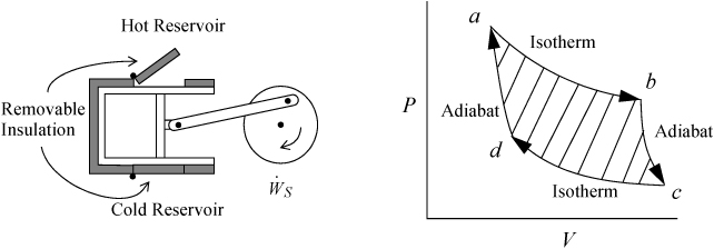
Figure 3.1. Schematic of the Carnot engine, and the Carnot P-V cycle when using a gas as the process fluid.
![]() The Carnot cycle is one method of constructing a heat engine.
The Carnot cycle is one method of constructing a heat engine.
Nicolas Léonard Sadi Carnot (1796–1832) was a French scientist who developed the Carnot cycle to demonstrate the maximum conversion of heat into work.
Let us consider the energy balance for the gas in the piston. Because the process is cyclic and returns to the initial state, the overall change in U is zero. The system is closed, so no flow work is involved. This work performed, WEC = ∫PdV for the gas, is equal to the work done on the shaft plus the expansion/contraction work done on the atmosphere for each step. By summing the work terms for the entire cycle, the net work done on the atmosphere in a complete cycle is zero since the net atmosphere volume change is zero. Therefore, the work represented by the shaded portion of the P-V diagram is the useful work transferred to the shaft.

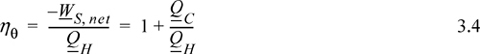
You can see from the shaded area in Fig. 3.1 that –WS, net > 0; therefore, since QH > 0 and QC < 0, ![]() . The ratio
. The ratio ![]() is negative, and to maximize η we seek to make QC as small in magnitude as possible.
is negative, and to maximize η we seek to make QC as small in magnitude as possible.
The heat transferred and work performed in the various steps of the process are summarized in Table 3.1. For this calculation we assume the gas within the piston follows the ideal gas law with temperature-independent heat capacities. We calculate reversible changes in the system; thus, we neglect temperature and velocity gradients within the gas (or we perform the process very slowly so that these gradients do not develop).
Table 3.1. Illustration of Carnot Cycle Calculations for an Ideal Gas.a
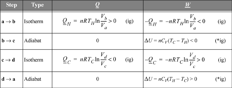
a. The Carnot cycle calculations are shown here for an ideal gas. There are no requirements that the working fluid is an ideal gas, but it simplifies the calculations.
Note: The temperatures TH and TC here refer to the hot and cold temperatures of the gas, which are not required to be equal to the temperatures of the reservoirs for the Carnot engine to be reversible. In Chapter 4 we will show that if these temperatures do equal the reservoir temperatures, the work is maximized.
Comparing adiabats b → c and d → a, the work terms must be equal and opposite since the temperature changes are opposite. The temperature change in an adiabatic process is related to the volume change in Eqn. 2.63. In that equation, when the temperature ratio is inverted, the volume ratio is inverted. Therefore, we reason that for the two adiabatic steps, Vb/Va = Vc/Vd. Using the ratio in the formulas for the isothermal steps, the ratio of heat flows becomes
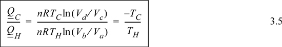
Inserting the ratio of heat flows into Eqn. 3.4 results in the thermal efficiency.
![]() The thermal efficiency of a heat engine is determined by the upper and lower operating temperatures of the engine.
The thermal efficiency of a heat engine is determined by the upper and lower operating temperatures of the engine.

You must use absolute temperature when applying Eqn. 3.6. We can skip the conversion to absolute temperature in the numerator of the last term because the subtraction means that the 273.15 (for units of K) in one term is canceled by the other. There is no such cancellation in the denominator.
Eqn. 3.6 indicates that we cannot achieve ηθ = 1 unless the temperature of the hot reservoir becomes infinite or the temperature of the cold reservoir approaches 0 K. Such reservoir temperatures are not practical for real applications. For real processes, we typically operate between the temperature of a furnace and the temperature of cooling water. For a typical power-plant cycle based on steam as the working fluid, these temperatures might be 900 K for the hot reservoir and 300 K for the cold reservoir, so the maximum thermal efficiency for the process is near 67%, theoretically. Most real power plants operate with thermal efficiencies closer to 30% to 40% owing to inherent inefficiencies in real processes.
Perspective on the Heat Engine
The Carnot cycle provides a quick and convenient guideline for processes that seek to convert heat flow into work. The striking conclusion we will prove in Chapter 4 is that it is impossible to convert all of the heat flow from the hot reservoir into work at reasonable temperatures. From an overall perspective, the detailed steps of the Carnot engine can be ignored. The amount of work is given by Eqn. 3.6. We can simply state that heat comes in, heat goes out, and the difference is the net work. This situation is represented by Fig. 3.2(a). As an alternate perspective, any process with a finite temperature gradient should produce work. If it does not, then it must be irreversible, and “wasteful.” This situation is represented by Fig. 3.2(b). These observations are similar to previous statements about gradients and irreversibility, but Eqn. 3.6 establishes a quantitative connection between the temperature difference and the reversible work possible.

Figure 3.2. The price of irreversibility. (a) Overall energy balance perspective for the reversible heat engine. (b) Zero work production in a temperature gradient without a heat engine, QH = QC.
We will demonstrate in Chapter 4 that the Carnot thermal efficiency matches the upper limit attainable by any feasible process using heat flow as the source of work. On the other hand, it is not necessarily true that every engine is a heat engine. For instance, a fuel cell could conceivably convert the chemical energy of gasoline into electricity and then power a motor from the electricity. Fuel cells are not bound by the constraints of the Carnot cycle because they are not dependent on heat as the energy source. Also, not all engines operate between constant temperature reservoirs, so the direct comparison with the Carnot cycle is not possible.
Carnot Heat Pump
Suppose that we decided to reverse every step in the Carnot cycle. All the state variables would be the same, but all the heat and work flows would change signs. Instead of producing work, the process would require work, but it would absorb heat from a cold reservoir and reject heat to a warm reservoir. A Carnot heat pump may be used as a refrigerator/freezer or as a heater depending on whether the system of interest is on the cold or warm side of the heat pump. In a refrigeration system, the goal is to remove heat from the cold area and reject it to the warmer surroundings. Heat pumps can be purchased for home heating, and in that mode, they can extract heat from the colder outdoors and “pump” it to the warmer house.
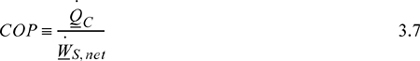
For a given transfer of heat from the cold reservoir, a Carnot heat pump requires the minimum amount of work for any conceivable process. The coefficient of performance, COP, is the ratio of heat transferred from the cold reservoir to the work required. COP is a mirror image of thermal efficiency, reappearing in Units I and II. We want to maximize COP when the objective is to cool a refrigerator with as little work as possible.
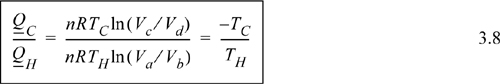
Eqn. 3.5 has a subtle inversion of volumes that drops out:
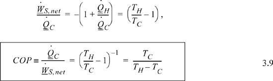
Eqn. 3.3 still applies, and the COP is given by
Example 3.1. Analyzing heat pumps for housing
Suppose your family is considering replacing your furnace with a heat pump. Work is necessary in order to “pump” the heat from the low outside temperature up to the inside temperature. The best you could hope for is if the heat pump acts as a reversible heat pump between a heat source (outdoors in this case) and the heat sink (indoors). The average winter temperature is 4°C, and the building is to be maintained at 21°C. The coils outside and inside for transferring heat are of such a size that the temperature difference between the fluid inside the coils and the air is 5°C. We generally refer to this as the approach temperature. What would be the maximum cost of electricity in ($/kW-h) for which the heat pump would be competitive with conventional heating where a fuel is directly burned for heat. Consider the cost of fuel as $7.00 per 109J, and electricity as $0.10 per kW-h. Consider only energy costs.
Solution
The Carnot heat pump COP, Eqn. 3.9
where ![]() is the heating requirement in kW. Heat pump operating
is the heating requirement in kW. Heat pump operating ![]() , where θ is an arbitrary time and x is the cost.
, where θ is an arbitrary time and x is the cost.
Direct heating operating ![]() For the maximum cost of electricity for competitive heat pump operation, let heat pump cost = direct heating cost at the breakeven point.
For the maximum cost of electricity for competitive heat pump operation, let heat pump cost = direct heating cost at the breakeven point.
Since the actual cost of electricity is given as $0.10/kW-h it might be worthwhile if the heat pump is reversible and does not break down. (Purchase, installation, and maintenance costs have been assumed equal in this analysis, although the heat pump is more complex.)
3.2. Distillation Columns
Roughly 80% of separations are conducted by distillation and a significant portion of the energy involved in the global chemical process industries is devoted to distillation. Why are more distillation columns needed than reactors? Reactors rarely run to 100% conversion and rarely produce a single product with 100% purity. There may be a by-product of the primary reaction or a solvent reaction medium. Additionally, there may be side reactions that can be minimized but not eliminated. Altogether, the reactor effluent almost always contains several components, and products need to be separated to high purity before they can be sent out of the process or recycled.
Analyzing distillation is important for a more philosophical reason as well. It is a common unit operation that involves mass and energy balances, heat and mass transfer, and phase partitioning. This kind of analysis pervades chemical engineering in general. The important consideration is the thought process that leads to the model equations. That thought process can be applied to any system, no matter how complex. As we proceed through the analysis distillation, try to imagine how you might develop similar approximations for other systems. Challenge yourself to anticipate the next step in every derivation. In the final analysis, your skill at developing simple models of complex phenomena is more valuable than memorizing model equations developed by somebody else.
We will address the phase equilibrium aspects of distillation in Section 10.6 on page 390, and you may wish to skim that section now. Briefly, the fraction with the lowest boiling point rises in the column and the fraction with the highest boiling point flows to the bottom. In this section, the focus is on mass and energy balances for distillation. A common model in distillation column screening is called constant molar overflow. In this model, the actual enthalpy of vaporization of a mixture is represented by the average enthalpy of vaporization, which can be assumed to be independent of composition for the purposes of this calculation, ![]() . Also, all saturated liquid streams are considered to have the same enthalpy, and all saturated vapor streams are considered to have the same enthalpy. These assumptions may seem extreme, but the model provides an excellent overview of key operating conditions.
. Also, all saturated liquid streams are considered to have the same enthalpy, and all saturated vapor streams are considered to have the same enthalpy. These assumptions may seem extreme, but the model provides an excellent overview of key operating conditions.
In the constant molar overflow model for a column with one feed, the column may be represented by five sections as shown in Fig. 3.3: a feed section where the feed enters; a rectifying section above the feed zone; a condenser above the rectifying section which condenses the vapors and returns a portion of the liquid condensate as reflux LR to ensure that liquid remains on the trays to induce the liquid-vapor partitioning that enhances the compositions.; a stripping section below the feed section; and a reboiler that creates vapors from the liquid flowing down the column.
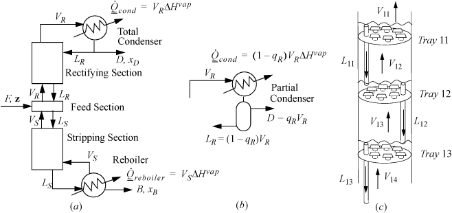
Figure 3.3. (a) Overall schematic of a distillation column with a total condenser showing five sections of a distillation column. and conventional labels; (b) a partial condenser; (c) schematic of liquid levels on bubble cap trays with the downcomers used to maintain the liquid levels.
At the bottom of the column, heat is added in the reboiler, causing vapor to percolate up the column until it reaches the condenser. The heat requirement in the reboiler is called the heating duty. B is called the bottoms or bottoms product. The ratio VS/B is called the boilup ratio. The energy requirement of the reboiler is known as the reboiler duty and is directly proportional to the moles of vapor produced as shown in the figure.
At the top of the column, Fig. 3.3(a) shows a total condenser where the vapor from the top of the column is totally condensed. The liquid flow rate leaving the condenser will be VR = (LR + D). D is called the overhead product or distillate. LR is called the reflux. The proportion of reflux is characterized by the reflux ratio, R = LR/D. A partial condenser may also be used as shown in (b), and the overhead product leaves as a vapor and the condensed fraction is the reflux. The cooling requirement of the condenser is called the condenser duty and the duty depends on whether the condenser is total or partial as shown in the figure.
The rectifying and stripping sections of the column have either packing or trays to provide retention of the liquid and contact with vapors. Trays are easier to introduce as shown in Fig. 3.3(c). At steady state, each tray holds liquid and the vapor flows upwards through the liquid. The trays can be constructed with holes (sieve trays) or bubble caps (bubble cap trays) or valves (valve trays). The bubble caps sketched in the figure represent a short stub of pipe with a short inverted “cup” called the “cap” with slots in the sides (slots are not shown) supported with spacing so that vapor can flow upwards through the pipe and out through the slots in the cap. A downcomer controls the liquid level on the tray as represented by a simple pipe extending above the surface of the tray in the figure. and in an ideal column each tray creates a separation stage. Using multiple stages provides greater separation. By stacking the stages, rising vapor from a lower stage boils the liquid on the next stage. At steady state, streams VS and VR are assumed to be saturated vapor unless otherwise noted. Streams B, LS, and LR are assumed to be saturated liquid unless otherwise noted. D is either assumed to be either a saturated liquid or a vapor depending on whether the condenser is total or partial, respectively. According to the constant molar overflow model, at steady state the vapor and liquid flow rates are constant within the stripping and rectifying sections because all the internal streams in contact are saturated, and change only at the feed section as determined by mass and energy balances around the feed section.
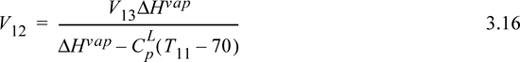
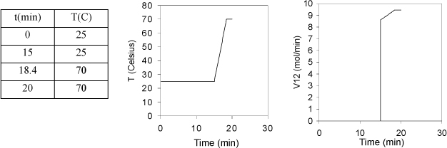
One of the most challenging tasks in the undergraduate chemical engineering laboratory is to explain the dynamics of the distillation column during start-up. Students tend to assume that the entire distillation column starts working as soon as heat is applied to the reboiler. However, during column start-up, the internal flows are not constant in the column sections. Heat moves up the column one tray at a time as boiling vapor leaves one tray and enters another. Consider Fig. 3.3(c). When tray 12 starts to boil, rising vapors will be condensed by the cold liquid on tray 11 immediately above and by the cold column. In principle, the vapor flow leaving the upper tray 11, V11, will be approximately zero until the column and liquid on the tray reaches the saturation temperature of the liquid on tray 11. Vapors reaching tray 11 are condensed and give up latent heat. Then tray 11 begins to warm. The condensed vapors create liquid overflow of subcooled liquid from tray 11 back down to tray 12. The lower tray 12 continues to boil, but the cool downcomer liquid causes the vapor rate V12 to be smaller than V13. Tray 12 stays at a fairly constant temperature as it continues to boil because it stays saturated. Finally, when tray 11 begins to boil, the process repeats for tray 10 and so on.
This introduction is not intended to explain every detail of distillation and energy balances, but it should suffice for you to deduce the most important qualitative behaviors. An illustration of the kinds of possible inferences is given in Example 3.2. Homework problem 3.4 provides additional exercises related to steady-state distillation.
Example 3.2. Start-up for a distillation column
A particular bubble cap distillation column for methanol + water has 12 trays numbered from top to bottom. Each tray is composed of 4 kg of materials and holds 1 kg of liquid. The heat capacity of the tray materials is 6 J/g-K and the heat capacity of the liquid is 84 J/mol-K = 3.4 J/g-K. During start-up, the feed is turned off. Roughly 15 minutes after the reboiler is started, tray 12 has started to boil and the temperature on tray 11 begins to rise. The reboiler duty is 6 kW and the heat loss is negligible. Tray 11 starts at 25 °C and the temperature of the liquid and the tray materials is assumed the same during start-up. Assume the liquid inventory on Tray 11 is constant throughout start-up.
a. Tabulate and plot the temperature versus time for tray 11 until it starts to boil at 70 °C.
b. Plot the vapor flow V12 as a function of time.
Solution
a. First, recognize that V11 = 0 since tray 11 is subcooled. No liquid is flowing down to tray 11. L10 = 0 since F = 0 and no vapors are being condensed yet (LR = 0), even though the cooling water may be flowing.
Mass balance on tray 11 (all vapors from below are being condensed during start-up, V11 = 0, L10 = 0):
Mass balance on boundary around tray 11 + tray 12 (V11 = 0, L10 = 0, during start-up):
State 11 is subcooled during start-up and will warm until T11 = 70:
Energy balance on tray 11 during start-up (no work, no direct heat input, energy input by flow of hot vapors, negligible heat loss):
where for the last equality we have inserted Eqn. 3.10 and then Eqn. 3.12.
An energy balance on tray 12 (which is at constant temperature) gives:
Using Eqn. 3.12 to eliminate H11, Eqn. 3.10 to eliminate L11, and Eqn. 3.11 to eliminate L12,
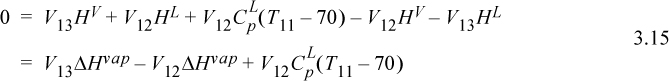
Inserting Eqn. 3.15 into Eqn. 3.13, and recognizing the constant vapor flow rate below tray 13,
where ‘mat’ indicates column material. Inserting values from the problem statement gives,
The tray will require approximately (70 – 25)/13.1 = 3.4 min to reach saturation temperature. The plot is shown below.
b. The vapor flow is given by Eqn. 3.13 using T11 = 25 + 13.1(t – 15). The average heat of vaporization is (40.7 + 35/3)/2 = 38 kJ/mol. Between 15 and 18.4 min, the flow rate in mol/min
Note that we neglect details like imperfect mixing or bypass heating (vapor that does not get condensed) that would round the edges of the temperature profile.
Note that as soon as vapors start to reach tray 11 in Example 3.2 the net energy input is constant even though the flow rate of hot vapors into the tray is increasing with time during start-up. Why? The answer is that energy is also being transported away from the tray by the flow down the downcomer. As the tray warms, this energy transport out is increasing at the same rate as the increased energy transport into the stage by the increasing flow of vapor. Analysis of subtleties such as this will deepen your understanding of physical phenomena and your appreciation for the utility of the energy balance.
3.3. Introduction to Mixture Properties
The previous section used “average” properties for the streams. This level of approximation is too crude for most calculations. We therefore need to understand how to estimate mixture properties.
Property Changes of Mixing
Communication of the property changes is facilitated by defining the property change of mixing as the mixture property relative to the mole-fraction weighted sum of the component properties in the unmixed state. Using x to be a generic composition variable, the energy of mixing is
The enthalpy of mixing is:
The volume of mixing is the volume of the mixture relative to the volumes of the components before mixing.
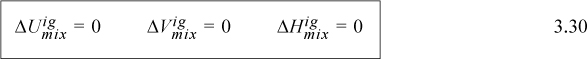
Similar equations may be written for other properties that we will define later: entropy of mixing, Gibbs energy of mixing, and Helmholtz energy of mixing – but these must reflect the increased disorder inherent in creating mixtures from pure fluids. If the property change on mixing (e.g., ΔHmix) has been measured and correlated in a reference book or database, we can use it to calculate the stream property at a later time:
3.4. Ideal Gas Mixture Properties
The ideal gas is a convenient starting point to introduce the calculation of mixture properties because the calculations are simple. Since ideal gas molecules do not have intermolecular potentials, the internal energy consists entirely of kinetic energy. When components are mixed at constant temperature and pressure, the internal energy is simply the sum of the component internal energies (kinetic energies), which can be written using y as a gas phase composition variable:
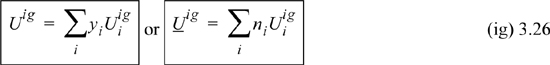
The total volume of a mixture is related to the number of moles by Amagat’s law:
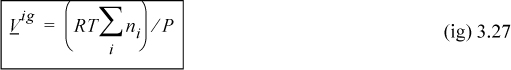
We can thus see that the energy of mixing and the volume of mixing for an ideal gas are both zero. Combining U and V to obtain the definition of H, H = U + PV, and using Eqns. 3.26 and 3.27,
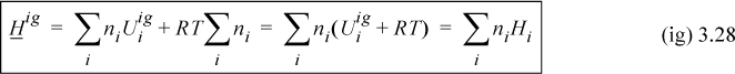
Therefore the enthalpy of a mixture is given by the sum of the enthalpies of the components at the same temperature and pressure and the enthalpy of mixing is zero. On a molar basis,
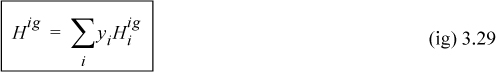
Furthermore, we can add the component enthalpies and internal energies for ideal gas mixtures using the mole fractions as the weighting factors. The energy of mixing, volume change of mixing, and enthalpy change of mixing are all zero.
3.5. Mixture Properties for Ideal Solutions
Sometimes the simplest analysis deserves more consideration than it receives. Ideal solutions can be that way. For an ideal solution, there are no synergistic effects of the components being mixed together; each component operates independently. Thus, mixing will involve no energy change and no volume change. Using x as a generic composition variable,
Though these restrictions were also followed by ideal gas solutions, the volumes for ideal solutions do not need to follow the ideal gas law, and can be liquids; thus, ideal gases are a subset of ideal solutions. Examples of ideal solutions are all ideal gases mixtures and liquid mixtures of family member pairs of similar size such as benzene + toluene, n-butanol + n-pentanol, and n-pentane + n-hexane.
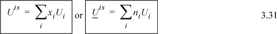
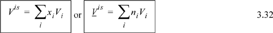
Since H ≡ U + PV, and because the U and V are additive, the enthalpy of the mixture will simply be the sum of the pure component enthalpies times the number of moles of that component:

Therefore, an ideal solution has a zero energy of mixing, volume of mixing, and enthalpy of mixing (commonly called the heat of mixing):

The primary distinction between ideal gas mixtures and ideal solutions is the constraint of the ideal gas law for the volume of the former. Let us apply the principles of ideal solutions and ideal gas mixtures to an example that also integrates the principles of use of a reference state.
Example 3.3. Condensation of a vapor stream
A vapor stream of wt fractions 45% H2O, 40% benzene, 15% acetone flows at 90°C and 1 bar into a condenser at 100 kg/h. The stream is condensed and forms two liquid phases. The water and benzene can be considered to be totally immiscible in one another. The acetone partitions between the benzene and water layer, such that the K-ratio, K = (wt. fraction in the benzene layer)/(wt. fraction in the water layer) = 0.9.a The liquid streams exit at 20°C and 1 bar. Determine the cooling duty, ![]() for the condenser. Assume the feed is an ideal gas and the liquid streams are ideal solutions once the immiscible component has been eliminated.
for the condenser. Assume the feed is an ideal gas and the liquid streams are ideal solutions once the immiscible component has been eliminated.
Solution
A schematic of the process is shown below. Using ![]() as the flow rate of acetone in E and
as the flow rate of acetone in E and ![]() as the flow rate in stream B, the K-ratio constraint is
as the flow rate in stream B, the K-ratio constraint is
where the acetone mass balance has been inserted in the second equality.
Using the first and third arguments, a quadratic equation results, which leads to ![]() , and
, and ![]() .
.

The energy balance for the process side of the dotted boundary is:
We are free to choose a reference state for each component. Note that if the reference state is chosen as liquid at 20°C, then the enthalpies of E and B will both be zero since they are at the reference state temperature and pressure and the enthalpy of mixing is zero for the ideal solution assumption. This choice will greatly reduce the number of calculations. The energy balance with this reference state simplifies to the following:
The enthalpy of F as an ideal gas is given by Eqn. 3.28:
Refer back to Fig. 2.6 on page 65 to review the paths for calculation relative to a reference state. The path used here is similar to Fig. 2.6(a). To calculate the enthalpy for components in F, we can construct a path between the reference state and the feed state going through the normal boiling point, Tb, where the heat of vaporization is known.
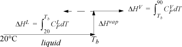
The enthalpy of a component in the feed stream is a sum of the three steps, Hi,F = ΔHL + ΔHvap + ΔHV. Note that Tb > 90°C for water. The ΔHV term is calculated with the same formula, but results in a negative contribution as shown by the dotted line in the path calculation schematic. For benzene and acetone, Tb < 90°C, so the path shown by the solid line is used for ΔHV. Note that, although the system is below the normal boiling point of water at 1 bar, the water can exist as a component in a mixture.
Using the heat capacity polynomials, and tabulating the three steps shown in the pathway schematic, programming the enthalpy integrals into Excel or MATLAB provides
HF, H2O = 6058 + 40656 – 342 = 46372 J/mol
HF, benz = 8624 + 30765 + 994 = 40383 J/mol
HF, acet = 4639 + 30200 + 2799 = 37638 J/mol
Note that the last term in the sum is negative for water because the feed temperature of the mixture is below the normal boiling temperature. The cooling duty for the condenser is
a. Throughout most of the text, we usually use K-ratios based on mole fraction ratio, not weight fraction. Nevertheless, many references use K-ratios based on weight fractions. You must read carefully and convert as needed.
3.6. Energy Balance for Reacting Systems
Chemical engineers must be proficient at including reacting systems into energy balances, and there are several key concepts that must be introduced. In reacting systems the number of moles is not conserved unless the number of moles of products is the same as the number of moles of reactants. Generally, the two best approaches for tracking species are to use an atom balance or to use the reaction coordinate. Here we will introduce the method of the reaction coordinate because it is much easier to incorporate into the energy balance. It is convenient to adopt the conventions of stoichiometry,
v1C1 + v2C2 + v3C3 + v4C4 = 0
where the C’s represent the species, and reactants have negative v’s and products have positive v’s. The v’s are called the stoichiometric numbers, and the absolute values are called the stoichiometric coefficients. (e.g., CH4 + H2O ![]() CO + 3H2, numbering from left to right),
CO + 3H2, numbering from left to right),
⇒ v1 = –1; v2 = –1; v3 = +1; v4 = +3.
Consider what would happen if a certain amount of component 1 were to react with component 2 to form products 3 and 4. We see dn1 = dn2 (v1 / v2) because v1 moles of component 1 requires v2 moles of component 2 in order to react. Rearranging:

Since all these quantities are equal, it is convenient to define a variable which represents this quantity.
ξ is called the reaction coordinate1 and is related to the conversion.2 Integrating:
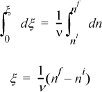
Or in a more useful form for any component i:

In a flowing system, ![]() represents the outlet,
represents the outlet, ![]() represents the inlet, and thus for component i,
represents the inlet, and thus for component i,
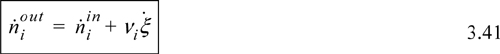
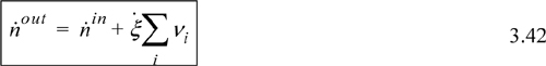
where ![]() represents the overall rate of species interconversion. Moles are not conserved in a chemical reaction, which can be quantified by summing Eqn. 3.40 or 3.41 over all species—for a flowing system,
represents the overall rate of species interconversion. Moles are not conserved in a chemical reaction, which can be quantified by summing Eqn. 3.40 or 3.41 over all species—for a flowing system, ![]() and
and ![]() , thus,
, thus,
In closed systems, the value of ξ is determined by chemical equilibria calculations; ξ may be positive or negative. The only limit on ξ is that ![]() for all i. The boundary values of ξ may be determined in this manner before beginning an equilibrium calculation. Naturally, in a flowing system, the same arguments apply to
for all i. The boundary values of ξ may be determined in this manner before beginning an equilibrium calculation. Naturally, in a flowing system, the same arguments apply to ![]() and
and ![]() .
.
Example 3.4. Stoichiometry and the reaction coordinate
Five moles of hydrogen, two moles of CO, and 1.5 moles of CH3OH vapor are combined in a closed system methanol synthesis reactor at 500 K and 1 MPa. Develop expressions for the mole fractions of the species in terms of the reaction coordinate. The components are known to react with the following stoichiometry:
2H2(g) + CO(g) ![]() CH3OH(g)
CH3OH(g)
Although the reaction is written as though it will proceed from left to right, the direction of the actual reaction does not need to be known. If the reverse reaction occurs, this will be obvious in the solution because a negative value of ξ will be found. The task at hand is to develop the mole balances that would be used toward determining the value of ξ. The table below presents a convenient format.
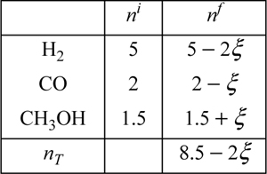
The total number of moles at any time is 8.5 – 2ξ. The mole fractions are
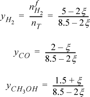
To ensure that all ![]() , the acceptable upper limit of ξ is determined by CO, and the acceptable lower limit is determined by CH3OH,
, the acceptable upper limit of ξ is determined by CO, and the acceptable lower limit is determined by CH3OH,
–1.5 ≤ ξ ≤ 2
Example 3.5. Using the reaction coordinates for simultaneous reactions
For each independent reaction, a reaction coordinate variable is introduced. When a component is involved in two reactions, the moles are related to both reaction coordinates. This example is available as an online supplement.
Standard State Heat of Reaction
When a reaction proceeds, bonds are broken, and others are formed. Because the bond energies vary for each type of bond, there are energy and enthalpy changes on reaction. Bond changes have a significant effect on the energy balance because they are usually larger than the sensible heat effects. Because enthalpies are state properties, we can use Hess’s law to calculate the enthalpy change. Hess’s law states that the enthalpy change of a reaction can be calculated by summing any component reactions, or by calculating the reaction enthalpy along a convenient reaction pathway between the reactants and products. To organize calculations of the changes, enthalpies of components are usually available at a standard state. A standard state is slightly different from a reference state as discussed on page 63. A standard state requires all the specifications of a reference state, except the T is the temperature of the system. For reactions, the conventional standard state properties are at a specified composition, state of aggregation, and pressure, but they change with temperature. By combining Hess’s law with the standard state concept, we may calculate the standard state heat (or enthalpy) of reaction. Suppose that we have the reaction of Fig. 3.4. For calculation of the heat of reaction, a convenient pathway is “decompose” the reactants into the constituent elements in their naturally occurring states at the standard state conditions, and then “reform” them into the products. The enthalpy of forming each product from the constituent elements is known as the standard heat (or enthalpy) of formation. The enthalpy change for “decomposing” the reactants is the negative of the heat of formation.
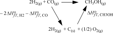
Figure 3.4. Illustration of the calculation of the standard heat of reaction by use of standard heats of formation.
We may write this mathematically using the stoichiometric numbers as:

where every term in the equation varies with temperature. Frequently, the standard state pressure is 1 bar. When a reaction is not at 1 bar, the usual practice is to incorporate pressure effects into the energy balance as we will show later, rather than using a heat of reaction at the high pressure. If we specify a reference temperature in addition to the other properties used for the standard state, we can calculate the ![]() at any temperature by using the heat capacity of the reactants and products,
at any temperature by using the heat capacity of the reactants and products,

where ![]() . A reaction with a negative value of
. A reaction with a negative value of ![]() is called an exothermic reaction. A reaction with a positive value of
is called an exothermic reaction. A reaction with a positive value of ![]() is called an endothermic reaction. In this equation,
is called an endothermic reaction. In this equation, ![]() is easily determined if the standard heat of reaction
is easily determined if the standard heat of reaction ![]() is known at a single reference temperature and 1 bar.
is known at a single reference temperature and 1 bar.

This is Eqn. 3.43, with an additional specification of temperature which creates a reference state. Almost always, the best reference state to use is TR = 298.15 K and 1 bar, because this is the temperature where the standard state enthalpies (heats) of formation are commonly tabulated. The heat of formation is taken as zero for elements that naturally exist as molecules at 298.15 K and 1 bar. Then the zero value is set for the state of aggregation naturally occurring at 298.15 K and 1 bar. For example, H exists naturally as H2(g), so ![]() is zero for H2(g). Carbon is a solid, so the value of
is zero for H2(g). Carbon is a solid, so the value of ![]() is zero for C(s). The zero values for elements in the naturally occurring state are often omitted in the tables in reference books. Enthalpies of formation are tabulated for many compounds in Appendix E at 298.15 K and 1 bar.
is zero for C(s). The zero values for elements in the naturally occurring state are often omitted in the tables in reference books. Enthalpies of formation are tabulated for many compounds in Appendix E at 298.15 K and 1 bar.
The state of aggregation must be specified in the reaction and care should be used to obtain the correct value from the tables. Some molecules, like water, commonly exist as vapor (g), or liquid (l). Note that for water, the difference between ![]() and
and ![]() is nearly the heat of vaporization at 298.15 K that can be obtained from the steam tables except that a minor pressure correction has been applied to correct the values from the vapor pressure to 1 bar.
is nearly the heat of vaporization at 298.15 K that can be obtained from the steam tables except that a minor pressure correction has been applied to correct the values from the vapor pressure to 1 bar.
The full form of the integral of Eqn. 3.44 is tedious to calculate manually, e.g., if CP, i = ai + bi T + ci T2 + di T3, Eqn. 3.44 becomes
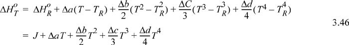
where ![]() , and heat capacity constants b, c, and d are handled analogously. The value of the constant J is found by using a known numerical value of ΔHRo in the upper equation (e.g., 298.15K) and setting the temperature to TR.
, and heat capacity constants b, c, and d are handled analogously. The value of the constant J is found by using a known numerical value of ΔHRo in the upper equation (e.g., 298.15K) and setting the temperature to TR.
Energy Balances for Reactions
To calculate heat transfer to or from a reactor system, the energy balance used in earlier chapters requires further consideration. To simplify the derivation of the energy balance for reactive systems, consider a single inlet stream and single outlet stream flowing at steady state:
For either the inlet stream or the outlet stream, the total enthalpy can be calculated by summing the enthalpy of the components plus the enthalpy of mixing at the stream temperature and pressure. To properly use Eqn. 3.47, the enthalpies of the inlets and outlets need to be related to the reaction. Two methods are used for energy balances, and both are equally valid. An overview of the concept pathways is illustrated in Fig. 3.5. To make a thermodynamic connection with the reaction, the Heat of Reaction method replaces the first two terms in Eqn. 3.47 with the negative sum of the three steps shown by dashed lines in Fig. 3.5(a). In contrast, the Heat of Formation method uses an elemental reference state for every component, and the enthalpies of each component include the heat of formation as illustrated by each branch of Fig 3.5(b). The difference of enthalpies of the components then includes the generalized steps of Fig. 3.4, and the heat of reaction is included implicitly when taking the difference in the two branches of Eqn. 3.5(b). The difference in the two branches represents the first two terms of Eqn. 3.47. The Heat of Reaction method is usually easiest for students to grasp, because of the explicit term for the heat of reaction. An advantage of the method is that an experimental heat of reaction can be readily used. Most process simulators use the Heat of Formation method. If you think about it, the Heat of Formation method does not require specification of exactly what reactions occur. Based on Hess’s law, the overall results can be related to the differences in the heats of formation of the outlet and the inlet species. The notation and the manipulated energy balances for the two methods look different, and the choice of the method depends on data available. The numerical results are the same if the thermochemical data are reliable for each method. Differences will be due to accuracies in the properties used for the pathways.

Figure 3.5. Concept pathways for (a) the Heat of Reaction method and (b) the Heat of Formation method. Details for the steps are omitted as discussed in the text.
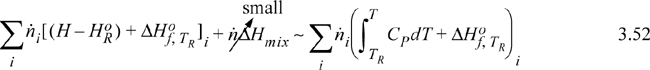
Either method requires manipulation of stream enthalpies relative to the reference conditions. When discussing reference states in Section 2.11, convenient pathways were used. The reaction balance calculations require that the inlets and outlets be related to the standard state TR and Po using similar techniques, and often phase changes are necessary. Following our convention of hierarchical learning, we will use a simplified balance that ignores some of these terms (which are frequently small corrections anyway relative to the heat of reaction). In later chapters, we introduce methods to calculate them. By comparing the magnitude of terms for a particular application, you will then be able to evaluate their relative importance. Choices can be made for the route to calculate a stream enthalpy. One choice is to mix all the components at an ideal gas state and then correct for non-idealities of the mixture. Another route is to correct for non-ideal gas behavior of individual components, and then mix them together at the system T and P. For a system without phase transitions between TR and T, when calculating the mixing process after the pressure correction, the stream enthalpy relative to species at the standard state looks like this,

where ![]() is the enthalpy of the species at the reference state, the pressure dependence of the enthalpy and the heat of mixing have been assumed to be small relative to the heat of reaction. Details on the pressure effects are developed in Chapters 6–8 and are expressed as an enthalpy departure; they are usually small relative to heats of reaction for gases. When the standard state is an ideal gas and liquid streams are involved, the correction is very important and –ΔHvap must be included in the path. The principle extends to solids as well. Heats of mixing are introduced beginning in Sections 11.4 and 11.10 and are typically small relative to reaction heats unless dissolving/neutralizing acids/bases or dissolving salts. Example 3.6 provides calculations including heats of vaporization for the components.
is the enthalpy of the species at the reference state, the pressure dependence of the enthalpy and the heat of mixing have been assumed to be small relative to the heat of reaction. Details on the pressure effects are developed in Chapters 6–8 and are expressed as an enthalpy departure; they are usually small relative to heats of reaction for gases. When the standard state is an ideal gas and liquid streams are involved, the correction is very important and –ΔHvap must be included in the path. The principle extends to solids as well. Heats of mixing are introduced beginning in Sections 11.4 and 11.10 and are typically small relative to reaction heats unless dissolving/neutralizing acids/bases or dissolving salts. Example 3.6 provides calculations including heats of vaporization for the components.
Heat of Reaction Method
It might not be immediately obvious that Eqn. 3.47 includes the heat of reaction. Considering just the flow terms of the energy balance, by plugging Eqn. 3.48 into Eqn. 3.47 the flow terms become
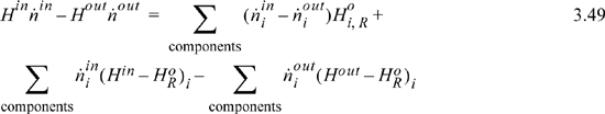
where the inlet temperature of all reactants is the same. The first term on the right of Eqn. 3.49 can be related to the heat of reaction using Eqn. 3.41 to introduce ξ and Eqn. 3.45 to insert the heat of reaction:

Therefore, the steady-state energy balance can be calculated using Eqn 3.51 and the balance is known as the Heat of Reaction method:
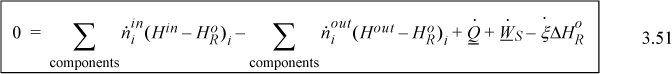
If you consider the first two terms and the last term, you can see how they represent the negative of the sum of the steps in Fig. 3.5(a). When multiple reactions occur, a reaction term can be used for each reaction. To use this expression correctly, the enthalpies of the inlet and outlet streams must be calculated relative to the same reference temperature where ![]() is known and any phase transitions at temperatures between the reference state and the inlet or outlet states must be included in
is known and any phase transitions at temperatures between the reference state and the inlet or outlet states must be included in ![]() . Also, the variable
. Also, the variable ![]() must be determined for the same basis as the molar flows. The temperature of 298.15 K is almost always the reference temperature for balances involving chemical reactions. There is less flexibility in choosing the reference temperature than for non-reactive systems. This method is easiest to apply with one or two reactions where the stoichiometry is known.
must be determined for the same basis as the molar flows. The temperature of 298.15 K is almost always the reference temperature for balances involving chemical reactions. There is less flexibility in choosing the reference temperature than for non-reactive systems. This method is easiest to apply with one or two reactions where the stoichiometry is known.
![]() An online supplement is available to relate the notation here to other common textbooks and includes other details.
An online supplement is available to relate the notation here to other common textbooks and includes other details.
Heat of Formation Method
The Heat of Formation method requires a reference state relative to the elements, and Eqn. 3.48 is modified by adding the heat of formation for each species. The stream enthalpy when there are no phase transitions between the reference state and the stream state looks like this:
![]() Enthalpy of a mixed stream where there are no phase changes between TR and T using the Heat of Formation method.
Enthalpy of a mixed stream where there are no phase changes between TR and T using the Heat of Formation method.
When phase changes are involved, the steps along the pathway are included as illustrated by several examples in Fig. Fig. 2.6 on page 65.
The energy balance is unmodified from Eqn. 3.47. The heat of reaction and the reaction coordinate are not needed explicitly, but the reaction coordinate is often helpful in determining the molar flows for the energy balance.
Work Effects
Usually shaft work and expansion/contraction work are negligible relative to other terms in the energy balance of a reactive system. They may usually be neglected without significant error.
Example 3.6. Reactor energy balances
Acetone (A) is reacted in the liquid phase over a heterogeneous acid catalyst to form mesityl oxide (MO) and water (W) at 80°C and 0.25 MPa. The reaction is 2A ![]() MO + W. Conversion is to be 80%. The heat capacity of mesityl oxide has been estimated to be CPL (J/mol-K) = 131.16 + 0.2710T(K), CPV (J/mol-K) = 72.429 + 0.2645T(K), and the acentric factor is estimated to be 0.356. Other properties can be obtained from Appendix E or webbook.nist.gov. Ignore pressure corrections and assume ideal solutions.
MO + W. Conversion is to be 80%. The heat capacity of mesityl oxide has been estimated to be CPL (J/mol-K) = 131.16 + 0.2710T(K), CPV (J/mol-K) = 72.429 + 0.2645T(K), and the acentric factor is estimated to be 0.356. Other properties can be obtained from Appendix E or webbook.nist.gov. Ignore pressure corrections and assume ideal solutions.

a. Estimate the heat duty for a steady-state reaction with liquid feed (100 mol/h) and liquid products. Use the Heat of Reaction method calculated using liquid heats of formation.
b. Estimate the heat duty for the same conditions as (a), but use the Heat of Formation method incorporating heats of formation of ideal gases and Eqn 2.45 to estimate heat of vaporization. (This method is used by process simulators.)
c. Repeat part (b) with the modification of using the experimental heat of vaporization.
d. Estimate the heat duty for the same conditions as (a), but use the Heat of Formation method incorporating the heat of formation of liquids.
a. For MO and A, ![]() , –249.4 kJ/mol respectively, from NIST. The liquid phase standard state heat of reaction is –221 – 285.8 – 2(–249.4) = –8 kJ/mol. Using a reference state of the liquid species at 298.15 K and 1 bar, the enthalpy of the each component is given by
, –249.4 kJ/mol respectively, from NIST. The liquid phase standard state heat of reaction is –221 – 285.8 – 2(–249.4) = –8 kJ/mol. Using a reference state of the liquid species at 298.15 K and 1 bar, the enthalpy of the each component is given by ![]() ; the results are {A, 7.265 kJ/mol}, {MO, 12.068}, {W, 4.161}. The mass balance for 100 mol/h A feed and 80% conversion gives an outlet of 100(1 – 0.8) = 20 mol/h A, then,
; the results are {A, 7.265 kJ/mol}, {MO, 12.068}, {W, 4.161}. The mass balance for 100 mol/h A feed and 80% conversion gives an outlet of 100(1 – 0.8) = 20 mol/h A, then, ![]() . The energy balance is
. The energy balance is ![]() , or
, or ![]()
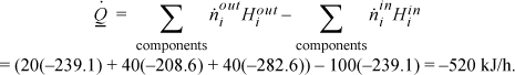
b. The value of ![]() is the same. The path to calculate the component liquid enthalpies using the heat of formation for ideal gases is: form ideal gas at 298.15K → heat ideal gas to 353.15K → condense ideal gas at 353.15K (using Eqn. 2.45). For MO
is the same. The path to calculate the component liquid enthalpies using the heat of formation for ideal gases is: form ideal gas at 298.15K → heat ideal gas to 353.15K → condense ideal gas at 353.15K (using Eqn. 2.45). For MO ![]() , from NIST. The enthalpies of each component will be tabulated for each of the three steps: (A) –215.7 + 4.320 – 27.71 = –239.1 kJ/mol; (MO) –178.3 + 8.72 – 39.0 = –208.6 kJ/mol; (W) –241.8 + 1.86 – 42.7 = –282.6 kJ/mol. The energy balance is
, from NIST. The enthalpies of each component will be tabulated for each of the three steps: (A) –215.7 + 4.320 – 27.71 = –239.1 kJ/mol; (MO) –178.3 + 8.72 – 39.0 = –208.6 kJ/mol; (W) –241.8 + 1.86 – 42.7 = –282.6 kJ/mol. The energy balance is
In principle, this method should have given the same result as (a), but the value differs significantly. The method is sensitive to the accuracy of the prediction for the heat of vaporization. When this method is used, the accuracy of the heat of vaporization needs to be carefully evaluated.
c. To evaluate the effect of the prediction of the heat of vaporization, let us repeat with a modified path through the normal boiling point of the species, using the experimental heat of vaporization. The normal boiling point of MO from NIST is 403 K, and ΔHvap = 42.7 kJ/mol. The component enthalpy path is modified to: form ideal gas at 298.15 K → heat ideal gas to Tb → condense to liquid at Tb → change liquid to 353.15 K. The enthalpies of each step and totals are: (A) –215.7 + 2.4 –30.2 + 3.3 = –240.2 kJ/mol; (MO) –178.3 + 17.3 – 42.7 – 11.6 = –215.3 kJ/mol; (W) –241.9 + 2.5 – 40.7 – 1.5 = –281.6 kJ/mol. The energy balance is
Parts (b) - (c) result in different heat transfer compared to (a). Note the difference in the heat of formation of vapor and liquid MO at 25°C matches the heat of vaporization at the normal boiling point and the difference would be expected to be larger. The original references for the thermochemical data should be consulted to decide which is most reliable.
d. This modification will not require heats of vaporization. The component enthalpy path is: form liquid at 298.15 K and heat liquid to 353.15 K. The sensible heat calculations are the same as tabulated in part (a). The enthalpies for the two steps and sum for each component are:
(A) –249.4 + 7.265 = –242.1 kJ/mol; (MO) –221 + 12.068 = –208.9; (W) –285.8 + 4.2 = –281.6.
The energy balance becomes:
Comparing with (a), the Heat of Formation method and the Heat of Reaction method give the same results when the same properties are used.
Adiabatic Reactors
Suppose that a reactor is adiabatic ![]() . For the Heat of Reaction method, the energy balance becomes (for a reaction without phase transformations between TR and the inlets or outlets),
. For the Heat of Reaction method, the energy balance becomes (for a reaction without phase transformations between TR and the inlets or outlets),
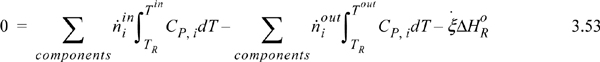
and as before, any latent heats must be added to the flow terms. An exothermic heat of reaction will raise the outlet temperature above the inlet temperature. For an endothermic heat of reaction, the outlet temperature will be below the inlet temperature. At steady state, the system finds a temperature where the heat of reaction is just absorbed by the enthalpies of the process streams. This temperature is known as the adiabatic reaction temperature, and the maximum reactor temperature change is dependent on the kinetics and reaction time, or on equilibrium. For fixed quantities and temperature of feed, Eqn. 3.53 involves two unknowns, Tout and ![]() , and, if the reaction is not limited by equilibrium, the kinetic model and reaction time determine these variables. If a reaction time is sufficiently large, equilibrium may be approached. Equilibrium reactors will be considered in Chapter 17.
, and, if the reaction is not limited by equilibrium, the kinetic model and reaction time determine these variables. If a reaction time is sufficiently large, equilibrium may be approached. Equilibrium reactors will be considered in Chapter 17.
Graphical Visualization of the Energy Balance
The energy balance as presented by Method I (Eqn. 3.51) can be easily plotted for an adiabatic reaction. Let us replace the heat capacity polynomials with average heat capacities that are temperature independent. If we incorporate the material balance, Eqn. 3.41, the Heat of Reaction steady-state energy balance after rearranging becomes
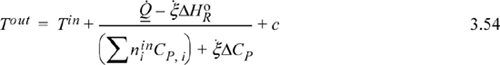
where ![]() and c is frequently small. Neglecting c and dropping heat for an adiabatic reactor,
and c is frequently small. Neglecting c and dropping heat for an adiabatic reactor,
Consider the case of an exothermic reaction. A schematic of the energy balance is shown in Fig. 3.6 for an exothermic reaction. In the plot, we have neglected ![]() in the denominator which is often small relative to the summation and introduces a slight curvature if included. Note that an endothermic reaction will have an energy balance with a negative slope, making the plot for an endothermic reaction a mirror image of Fig. 3.6 reflected across a vertical line at Tin.
in the denominator which is often small relative to the summation and introduces a slight curvature if included. Note that an endothermic reaction will have an energy balance with a negative slope, making the plot for an endothermic reaction a mirror image of Fig. 3.6 reflected across a vertical line at Tin.

Figure 3.6. Approximate energy balance for an adiabatic exothermic reaction. The dot represents the outlet reaction coordinate value and the adiabatic outlet temperature. The plot for an endothermic reaction will be a mirror image of this figure as explained in the text.
3.7. Reactions in Biological Systems
Living systems constantly metabolize food. In a sophisticated system such as a human, the digestive system breaks down the carbohydrates (sugars and starches), protein (complex amino acids), and fats (glycerol esters of fatty acids) into the building block molecules. There are exothermic reactions as the chemical structure of the food is modified by breaking bonds. The small molecules that result can be transported through the body as sugars, amino acids, and fatty acids. The body transforms these basic molecules to create energy to constantly replace cells and also to provide the energy needed for physical activity. The process more closely resembles fuel cell operation than a Carnot cycle, but the concepts of the energy balance still apply.
A major reaction providing energy in the human body is the oxidation of sugars and starches. These compounds are known to provide “quick energy” because they are easily burned. As an example, consider the oxidation of glucose to CO2 and H2O. Oxygen taken in through the lungs is carried to the cells where the reaction takes place. CO2 produced by the reaction is transported back to the lungs where it can be expelled. Water produced by the reaction largely is left as liquid, though respiration results in some transport. Although the actual process involves several intermediate steps, we know by Hess’s law that the overall energy and enthalpy change depends on only the initial and final structures, not the intermediate paths. The process for oxidation of glucose is
Like other combustion reactions, this reaction is exothermic. When intense physical activity occurs, the body is not able to use oxidation quickly enough to produce energy. In this case the body can convert glucose (or other sugars and starches) anaerobically to lactic acid as follows:
This is also an exothermic reaction, and there is no gas produced. This mechanism is used by muscles to provide energy and a build-up of lactic acid causes the muscular aching during and after vigorous exercise. Fats have higher energy content per mass and may be oxidized in a reaction analogous to Eqn. 3.56. Fat is used by the body to store energy. To burn fat, the body usually needs to be starved of the more easily metabolized starches and sugars.
The nervous system regulates body temperature so that when energy is burned, there is little change in body temperature. Some energy is transported out via respiration, some through evaporation of moisture through the skin, and some by heat transfer at the skin surface. Blood vessels in extremities are flexible and change size to regulate the blood flow, which is used to modify the flow rates. On a cold winter day, when our hands start to feel cold, our body is sensing a need to preserve body heat, so the vessels contract to decrease blood flow, making our hands feel even colder! During exercise, the vessels expand to increase cooling, and perspiration starts to provide evaporative cooling. In any event, our core temperature is maintained at 37°C as much as possible. When the body temperature drops the condition is called hypothermia. When the body is unable to eliminate heat, the condition is called hyperthermia and results in heat exhaustion and heat stroke. Usually, the body is able to regulate temperature, and the temperature is stable, so the body does not hold or loose energy by temperature changes. In an adult, the mass is also constant except for the daily cycles of eating and excretion that are very small perturbations of the total body mass.
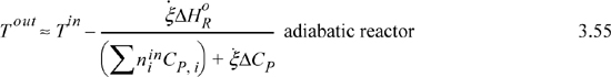
The body adjusts the metabolic rate as the level of physical activity changes. Data collected by performing energy balances on humans after 12 hours of fasting eliminate the heat effects due to digestion (about 30% higher) and provide an accurate measure of the metabolic rates. Examples of energy consumption are tabulated in Table 3.1.
Table 3.1. Summary of Energy Expenditure by Various Physical Activities for a 70 kg Persona
a. Vander, A.J., Serman, J.J., Luciano, D.S., 1985. Human Physiology: The Mechanisms of Body Function, 4th ed., ch. 15, New York: McGraw-Hill.
3.8. Summary
This chapter started by introducing the concept of heat engines and heat pumps to interconverted heat and work, and the limitations in efficiency. As a cyclic process, the systems are simple, but practice builds confidence in working with multistep processes. In the distillation section we introduced quite a few terms because there are a lot of flow rates in the sections of a distillation column. This section provided practice in working with choice of boundaries for balances and working with many streams. Sorting out the streams that are relevant is a key step in the solution of problems. We introduced ideal gas mixtures and ideal solutions, stressing that the energy of mixing and volume of mixing are zero for both and so the enthalpy of a stream is the sum of the enthalpies of the constituents. We then used reference states to solve an energy balance on a mixed stream including a phase transition. In the section on reacting systems we set forth the procedures to properly account for energy flows in and out of the system. Finally we demonstrated that the energy balance was relevant for complex biochemical reactions. The energy balance for a reaction is independent of whether it occurs biologically or in an industrial reactor. The goal of this section was to demonstrate the breadth of applications and to build your confidence in solving problems. At this point most students still do not have a grasp on reversibility and irreversibility, which should be clarified in the next chapter as we build on this material.
Important Equations
Two equations that come up repeatedly are the Carnot efficiency (Eqn. 3.6) and Carnot COP (Eqn. 3.9). The Carnot efficiency teaches that the conversion of heat energy into mechanical energy cannot be 100% efficient, even if every operation in the process is 100% efficient. This has major implications throughout modern society, reflected in limitations on power plants and energy management. Much of Units I and II is devoted to understanding the details of these kinds of problems and how to solve them more precisely. The Carnot thermal efficiency and COP are benchmarks for real processes, though real processes are not always operating between reservoirs. Common errors applying the formulas are: (1) to interchange the formulas and use the COP formula when you want the efficiency; and (2) to use relative temperature (°C or °F) instead of absolute temperature.
This chapter introduced the concept of ideal solutions and methods of solving energy balances with mixtures, including phase transitions. Important equations are
We also introduced the concept of the reaction coordinate and that all species in a single reaction can be related by
We finished with the energy balance, which is most often expressed in the approximate form for the Heat of Reaction method:

If the enthalpy of formation is incorporated into the enthalpy of the components, the Heat of Formation method looks unchanged from the energy balance of Chapter 2:
3.9. Practice Problems
P3.1. Dimethyl ether (DME) synthesis provides a simple prototype of many petrochemical processes. Ten tonnes (10,000 kg) per hour of methanol are fed at 25°C. The entire process operates at roughly 10 bar. It is 50% converted to DME and water at 250°C. The reactor effluent is cooled to 75°C and sent to a distillation column where 99% of the entering DME exits the top with 1% of the entering methanol and no water. This DME product stream is cooled to 45°C. The bottoms of the first column are sent to a second column where 99% of the entering methanol exits the top at 136°C, along with all the DME and 1% of the entering water, and is recycled. The bottoms of the second column exit at 179°C and are sent for wastewater treatment. Use the method of Example 3.6(b) to complete the following:
a. Calculate the enthalpy in GJ/h of the feed stream of methanol.
b. Calculate the enthalpy in GJ/h of the stream entering the first distillation column.
c. Calculate the enthalpy in GJ/h of the DME product stream.
d. Calculate the enthalpy in GJ/h of the methanol recycle stream.
e. Calculate the enthalpy in GJ/h of the aqueous product stream.
f. Calculate the energy balance in GJ/h of the entire process. Does the process involve a net energy need or surplus?
(ANS. -50, -106, -26, -51, -31, -7, i.e., energy surplus)
3.10. Homework Problems
3.1. Two moles of nitrogen are initially at 10 bar and 600 K (state 1) in a horizontal piston/cylinder device. They are expanded adiabatically to 1 bar (state 2). They are then heated at constant volume to 600 K (state 3). Finally, they are isothermally returned to state 1. Assume that N2 is an ideal gas with a constant heat capacity as given on the back flap of the book. Neglect the heat capacity of the piston/cylinder device. Suppose that heat can be supplied or rejected as illustrated below. Assume each step of the process is reversible.

a. Calculate the heat transfer and work done on the gas for each step and overall.
b. Taking state 1 as the reference state, and setting ![]() , calculate U and H for the nitrogen at each state, and ΔU and ΔH for each step and the overall Q and WEC.
, calculate U and H for the nitrogen at each state, and ΔU and ΔH for each step and the overall Q and WEC.
c. The atmosphere is at 1 bar and 298 K throughout the process. Calculate the work done on the atmosphere for each step and overall. (Hint: Take the atmosphere as the system.) How much work is transferred to the shaft in each step and overall?
3.2. One mole of methane gas held within a piston/cylinder, at an initial condition of 600 K and 5 MPa, undergoes the following reversible steps. Use a temperature-independent heat capacity of CP = 44 J/mol-K.
a. Step 1: The gas is expanded isothermally to 0.2 MPa, absorbing a quantity of heat QH1. Step 2: The gas is cooled at constant volume to 300 K. Step 3. The gas is compressed isothermally to the initial volume. Step 4: The gas is heated to the initial state at constant volume requiring heat transfer QH2. Calculate ΔU, Q, and WEC for each step and for the cycle. Also calculate the thermal efficiency that is the ratio of total work obtained to heat furnished, ![]() .
.
b. Step 1: The gas is expanded to 3.92 MPa isothermally, absorbing a quantity of heat QH1. Step 2: The gas is expanded adiabatically to 0.1 MPa. Step 3: The gas is compressed isothermally to 0.128 MPa. Step 4: The gas is compressed adiabatically to the initial state. Calculate ΔU, Q, WEC for each step and for the cycle. Also calculate the thermal efficiency for the cycle, ![]() .
.
3.3. The Arrhenius model of global warming constitutes a very large composite system.3 It assumes that a layer of gases in the atmosphere (A) absorbs infrared radiation from the Earth’s surface and re-emits it, with equal amounts going off into space or back to the Earth’s surface; 240 W/m2 of the solar energy reaching the Earth’s surface is reflected back as infrared radiation (S). The “emissivity value” (λ) of the ground (G) is set equal to that of A. λ characterizes the fraction of radiation that is not absorbed. For example, (1–λ) would be the fraction of IR radiation that is absorbed by the ground, and the surface energy would be S = Aλ + G(1–λ). A similar balance for the atmosphere gives, λG = 2λA. This balance indicates that radiation received from G is balanced by that radiated from A. The factor of 2 on the right-hand side appears because radiation can be toward the ground or toward space. The equations for radiation are given by the relations: G = σTG4 and A = σTA4 where σ = Stefan-Boltzmann constant 5.6704 x 10⁻⁸ (W/m2-K4).
a. Noting that the average TG is 300 K, solve for λ.
b. Solve for TG when λ = 0. This corresponds to zero global warming.
c. Solve for TG when λ = 1. This corresponds to perfect global warming.
d. List at least three oversimplifications in the assumptions of this model. Discuss whether these lead to underestimating or overestimating TG.
3.4. A distillation column with a total condenser is shown in Fig. 3.3. The system to be studied in this problem has an average enthalpy of vaporization of 32 kJ/mol, an average ![]() of 146 J/mol°-C, and an average
of 146 J/mol°-C, and an average ![]() of 93 J/mol°-C. Variable names for the various stream flow rates and the heat flow rates are given in the diagram. The feed can be liquid, vapor, or a mixture represented using subscripts to indicate the vapor and liquid flows, F = FV + FL. The enthalpy flow due to feed can be represented as: for saturated liquid, FLHsatL; for saturated vapor, FVHsatV; for subcooled liquid, FLHsatL + FLCPL(TF – TsatL); for superheated vapor, FVHsatV + FVCPV(TF – TsatV); and for a mix of vapor and liquid, FLHsatL + FVHsatV.
of 93 J/mol°-C. Variable names for the various stream flow rates and the heat flow rates are given in the diagram. The feed can be liquid, vapor, or a mixture represented using subscripts to indicate the vapor and liquid flows, F = FV + FL. The enthalpy flow due to feed can be represented as: for saturated liquid, FLHsatL; for saturated vapor, FVHsatV; for subcooled liquid, FLHsatL + FLCPL(TF – TsatL); for superheated vapor, FVHsatV + FVCPV(TF – TsatV); and for a mix of vapor and liquid, FLHsatL + FVHsatV.
a. Use a mass balance to show FV + VS – VR = LS – LR – FL.
[For parts (b)–(f), use the feed section mass and energy balances to show the desired result.]
b. For saturated vapor feed, FL = 0. Show VR = VS + FV, LS = LR.
c. For saturated liquid feed, FV = 0. Show VS = VR, LS = LR + FL.
d. For subcooled liquid feed, FV = 0. Show VR – VS = FLCP(TF – Tsat)/ΔHvap.
e. For superheated vapor feed, FL = 0. Show LS – LR = –FVCP(TF – Tsat)/ΔHvap.
f. For a feed mixture of saturated liquid and saturated vapor. Show VR = VS + FV, LS = LR + FL.
g. Use the mass and energy balances around the total condenser to relate the condenser duty to the enthalpy of vaporization, for the case of streams LR and D being saturated liquid.
h. Use the mass and energy balances around the reboiler to relate the reboiler duty to the enthalpy of vaporization.
i. In the case of subcooled liquid streams LR and D, the vapor flows out of the top of the column, and more variables are required. ![]() (into the condenser) will be smaller than the rectifying section flow rate VR. Also, the liquid flow rate in the rectifying section, LR, will be larger than the reflux back to the column,
(into the condenser) will be smaller than the rectifying section flow rate VR. Also, the liquid flow rate in the rectifying section, LR, will be larger than the reflux back to the column, ![]() . Using the variables
. Using the variables ![]() ,
, ![]() to represent the flow rate out of the top of the column and the reflux, respectively, relate VR to
to represent the flow rate out of the top of the column and the reflux, respectively, relate VR to ![]() ,
, ![]() and the degree of subcooling TL′, – TsatL.
and the degree of subcooling TL′, – TsatL.
[For parts (j)–(o), find all other flow rates and heat exchanger duties (Q values).]
j. F = 100 mol/hr (saturated vapor), B = 43, LR/D = 2.23.
k. F = 100 mol/hr (saturated vapor), D = 48, LS/VS = 2.5.
l. F = 100 mol/hr (saturated liquid), D = 53, LR/D = 2.5.
m. F = 100 mol/hr (half vapor, half liquid), B = 45, LS/VS = 1.5.
n. F = 100 mol/hr (60°C subcooled liquid), D = 53, LR/D = 2.5.
o. F = 100 mol/hr (60°C superheated vapor), D = 48, LS/VS = 1.5.
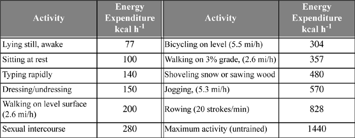
3.5. Allyl chloride (AC) synthesis provides a simple prototype of many petrochemical processes. 869 kg per hour of propylene (C3) are fed with a 1% excess of chlorine (Cl2) at 25°C. The entire process operates at roughly 10 bar. Cl2 is recycled to achieve a 50% excess of Cl2 at the reactor inlet. The reactor conversion is 100% of the propylene to AC and hydrochloric acid (HCl) at 511°C.
The reactor effluent is cooled to 35°C and sent to a distillation column where 98% of the entering AC exits the bottom with 1% of the entering Cl2 and no HCl. This AC product stream exits at 57°C. The tops of the first column are sent to a second column where 99% of the entering Cl2 exits the bottom at 36°C, along with 1% of the entering HCl, all of the AC, and is recycled. The tops of the second column exit at -31°C and are sent for waste treatment. Using the method of Heat of Formation method for the energy balance and ideal gas reference states with Eqn. 2.45 to estimate the heat of vaporization, complete the following.
a. Write a balanced stoichiometric equation for this reaction. (Hint: Check the NIST WebBook for chemical names and formulas.)
b. Perform a material balance to determine compositions and flow rates for all streams.
c. Using only streams (1), (6), (7), calculate the energy balance in MJ/h of the entire process. Does the process involve a net energy need or surplus?
d. Determine the heat load on the reactor in MJ/h.
e. Calculate the enthalpies in MJ/h of the feed stream 1.
f. Calculate the enthalpy in MJ/h of the stream 4 entering the first distillation column.
g. Calculate the enthalpy in MJ/h of the AC product stream 6.
h. Calculate the enthalpy in MJ/h of the Cl2 recycle stream 8.
i. Calculate the enthalpy in MJ/h of the HCl waste stream 7.
3.6. Chlorobenzene(l) is produced by reacting benzene(l) initially at 30°C with Cl2(g) initially at 30°C in a batch reactor using AlCl3 as a catalyst. HCl(g) is a by-product. During the course of the reaction, the temperature increases to 50°C. To avoid dichlorobenzenes, conversion of benzene is limited to 30%. On the basis of 1 mol of benzene, and 0.5 mol Cl2(g) feed, what heating or cooling is required using the specified method(s)? The NIST WebBook reports the heats of formation for liquid benzene and chlorobenzene at 25°C as 49 kJ/mol and 11.5 kJ/mol, respectively. The heat capacities of liquid benzene and chlorobenzene are 136 J/mol-K and 150 J/mol-K, respectively.
a. Use liquid reference states for the benzenes and the heat of reaction method for the energy balance.
b. Follow part (a), but instead, use the heat of formation method for the energy balance.
c. Use an ideal gas-phase reference state for the benzenes, Eqn. 2.45 to estimate the heat of vaporization, and the Heat of Reaction method.
3.7. Benzene and benzyl chloride produced from the reaction described in problem 3.6 are separated by distillation at 1 bar. The chlorine and HCl are removed easily and this problem concerns only a binary mixture. Suppose the liquid flow to the reboiler is 90 mol% chlorobenzene and 10 mol% benzene at 121.9°C. The boilup ratio is 0.7 at 127.8°C, and the vapor leaving the reboiler is 12.7 mol% benzene. The heat of vaporization of chlorobenzene is 41 kJ/mol. Heat capacities for liquids are in problem 3.6(a). Determine the heat duty for the reboiler.
3.8. In the process of reactive distillation, a reaction occurs in a distillation column simultaneously with distillation, offering process intensification. Consider a reactive distillation including the reaction: cyclohexene(l) + acetic acid(l) ![]() cyclohexyl acetate(l). In a reactive distillation two feeds are used, one for each reactant. In a small-scale column, the flows, heat capacities, and temperatures are tabulated below in mol/min. Assume the heat capacities are temperature-independent. All streams are liquids. Use data from the NIST WebBook for heats of formation to estimate the net heat requirement for the column.
cyclohexyl acetate(l). In a reactive distillation two feeds are used, one for each reactant. In a small-scale column, the flows, heat capacities, and temperatures are tabulated below in mol/min. Assume the heat capacities are temperature-independent. All streams are liquids. Use data from the NIST WebBook for heats of formation to estimate the net heat requirement for the column.

3.9. This problem considers oxidation of glucose as a model carbohydrate.
a. In the human body glucose is typically metabolized in aqueous solution. Ignoring the enthalpy change due to dissolving glucose in the aqueous solution, calculate the standard heat of reaction for Eqn. 3.56.
b. Using the standard heat of reaction calculated in part (a) together with the steady-state energy expenditure for sitting at rest, determine the rate that glucose is consumed (g/day). You may ignore sensible heats because the respiration streams are very close to 298.15 K.
c. Compare the energy consumption in part (b) with a light bulb by putting the energy consumption in terms of W, which is usually used to characterize light bulbs. How many 70 kg humans collectively produce energy equivalent to a 1500 W hair dryer?
d. On a mass basis, all carbohydrates have about the same heat of reaction. A soft drink has approximately 73 g carbohydrates (sugar) per 20 fluid oz. bottle and the manufacturer’s label reports that the contents provide 275 kcal. (Note: A dietary calorie is a thermodynamic kcal, so the conversion has already been made, and the bottle is labeled 275 calories.) Convert the answer from part (a) to kcal/g and compare with the manufacturer’s ratio.
e. What is the annual output of CO2 (kg) for a 70 kg human using the energy expenditure for sitting as an average value?
3.10. Compressed air at room temperature (295 K) is contained in a 20-L tank at 2 bar. The valve is opened and the tank pressure falls slowly and isothermally to 1.5 bar. The frictionless piston-cylinder is isothermal and isobaric (P = 1.5 bar) during the movement. The surroundings are at 1 bar. The volumes of the piping and valve are negligible. During the expansion, the piston is pushing on external equipment and doing useful work such that the total resistance to the expansion is equivalent to 1.5 bar. The entire system is then cooled until all of the air is back in the original container. During the retraction of the piston, the piston must pull on the equipment, and the resistance of the external equipment is equivalent to 0.1 bar, so the total force on the piston is less than 1 bar, 1.0 – 0.1 = 0.9 bar. The valve is closed and the tank is heated back to room temperature. (Air can be considered an ideal gas with a T-independent CP = 29 J/mol-K.)

a. The useful work done by the process is the total work done by the piston in the expansion step less the amount of work done on the atmosphere. Calculate the useful work done per expansion stroke in kJ.
b. Calculate the amount of heat needed during the expansion in kJ. Neglect the heat capacity of the tank and cylinder.
c. Calculate the amount of cooling needed during the retraction of the cylinder in kJ.
3.11. A well-insulated tank contains 1 mole of air at 2 MPa and 673 K. It is connected via a closed valve to an insulated piston/cylinder device that is initially empty. The piston may be assumed to be frictionless. The volumes of the piping and valve are negligible. The weight of the piston and atmospheric pressure are such that the total downward force can be balanced with gas pressure in the cylinder of 0.7 MPa. The valve between the tank and piston/cylinder is cracked open until the pressure is uniform throughout. The temperature in the tank is found to be 499.6 K. Air can be assumed to be an ideal gas with a temperature-independent heat capacity CP = 29.3 J/mol-K.
a. What is the number of moles left in the tank at the end of the process?
b. Write and simplify the energy balance for the process. Determine the final temperature of the piston/cylinder gas.
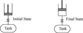
3.12. A piston/cylinder has two chambers and includes a spring as illustrated below. The right-hand side contains air at 20°C and 0.2 MPa. The spring exerts a force to the right of F = 5500x N where x is the distance indicated in the diagram, and xi = 0.3 m. The piston has a cross-sectional area of 0.1 m2. Assume that the piston/cylinder materials do not conduct heat, and that the piston/cylinder and spring do not change temperature. After oscillations cease, what is the temperature of the air in the right chamber and the final position of the piston, xf, for the cases listed below? Use a temperature-independent heat capacity for air, CP = 7R/2.
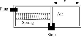
a. The left chamber is evacuated and the plug remains in place.
b. The plug is removed so that the left-side pressure stays at 0.1 MPa throughout the process.
3.13. We wish to determine the final state for the gas in an inflated balloon. Initially, the balloon has a volume of Vi at rest. The volume of the balloon is related to the internal pressure by V = a·P + b, where a and b are constants. The balloon is to be inflated by air from our lungs at Plung and Tlung which are known and assumed to remain constant during inflation. Heat transfer through the walls of the balloon can be ignored. The system is defined to be the gas inside the balloon at any time. Starting with the general energy balance, simplify to write the balance in terms of {CP, CV, Tlung, Plung, Ti, Tf, TR, PR} and either {Vi, Vf} or {Pi, Pf}. This will demonstrate that measurement of Vf or Pf is sufficient to determine Tf. Assume air is an ideal gas.