Chapter 8. Departure Functions
All the effects of nature are only the mathematical consequences of a small number of immutable laws.
P.-S. LaPlace
Maxwell’s relations make it clear that changes in any one variable can be represented as changes in some other pair of variables. In chemical processes, we are often concerned with the changes of enthalpy and entropy as functions of temperature and pressure. As an example, recall the operation of a reversible turbine between some specified inlet conditions of T and P and some specified outlet pressure. Using the techniques of Unit I, we typically determine the outlet T and q which match the upstream entropy, then solve for the change in enthalpy. Applying this approach to steam should seem quite straightforward at this stage. But what if our process fluid is a new refrigerant or a multicomponent natural gas, for which no thermodynamic charts or tables exist? How would we analyze this process? In such cases, we need to have a general approach that is applicable to any fluid. A central component of developing this approach is the ability to express changes in variables of interest in terms of variables which are convenient using derivative manipulations. The other important consideration is the choice of “convenient” variables. Experimentally, P and T are preferred; however, V and T are easier to use with cubic equations of state.
These observations combine with the observation that the approximations in equations of state themselves exhibit a certain degree of “fluidity.” In other words, the “best” approximations for one application may not be the best for another application. Responding to this fluidity requires engineers to revisit the approximations and quickly reformulate the model equations for U, H, and S. Fortunately, the specific derivative manipulations required are similar regardless of the equation of state since equations of state are either in the {T,P} or {T,V} form. The formalism of departure functions streamlines the each formulation.
An equation of state describes the effects of pressure on our system properties, including the low pressure limit of the ideal gas law. However, integration of properties over pressure ranges is relatively complicated because most equations of state express changes in thermodynamic variables as functions of density instead of pressure, whereas we manipulate pressure as engineers. Recall that our engineering equations of state are typically of the pressure-explicit form:
![]() Experimentally, P and T are usually specified. However, equations of state are typically density (volume) dependent.
Experimentally, P and T are usually specified. However, equations of state are typically density (volume) dependent.
and general equations of state (e.g., cubic) typically cannot be rearranged to a volume explicit form:
Therefore, development of thermodynamic properties based on {V,T} is consistent with the most widely used equations of state, and deviations from ideal gas behavior will be expressed with the density-dependent formulas for departure functions in Sections 8.1–8.5. In Section 8.6, we present the pressure-dependent form useful for the virial equation. In Section 8.8, we show how reference states are used in tabulating thermodynamic properties.
Chapter Objectives: You Should Be Able to...
1. Choose between using the integrals in Section 8.5 or 8.6 for a given equation of state.
2. Evaluate the integrals of Section 8.5 or 8.6 for simple equations of state.
3. Combine departure functions with ideal gas calculations to determine numerical values of changes in state properties, and use a reference state.
4. Solve process thermodynamics problems using a tool like Preos.xlsx or PreosProps.m rather than a chart or table. This skill requires integration of several concepts covered by other topical objectives including selection of the correct root, and reading/interpreting the output file.
8.1. The Departure Function Pathway
Suppose we desire to calculate the change in U in a process which changes state from (VL, TL) to (VH, TH). Now, it may seem unusual to pose the problem in terms of T and V, since we stated above that our objective was to use T and P. The choice of T and V as variables is because we must work often with equations of state that are functions of volume. The volume corresponding to any pressure is rapidly found by the methods of Chapter 7. We have two obvious pathways for calculating a change in U using {V, T} as state variables as shown in Fig. 8.1. Path A consists of an isochoric step followed by an isothermal step. Path B consists of an isothermal step followed by an isochoric step. Naturally, since U is a state function, ΔU for the process is the same by either path. Recalling the relation for dU(T,V), ΔU may be calculated by either.
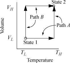
Figure 8.1. Comparison of two alternate paths for calculation of a change of state.
or Path B:
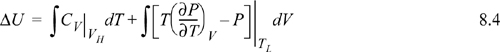
We have previously shown, in Example 7.6 on page 269, that CV depends on volume for a real fluid. Therefore, even though we could insert the equation of state for the integrand of the second integral, we must also estimate CV by the equation of state for at least one of the volumes, using the results of Example 7.6. Not only is this tedious, but estimates of CV by equations of state tend to be less reliable than estimates of other properties.
To avoid this calculation, we devise an equivalent pathway of three stages. First, imagine if we had a magic wand to turn our fluid into an ideal gas. Second, the ideal gas state change calculations would be pretty easy. Third, at the final state we could turn our fluid back into a real fluid. Departure functions represent the effect of the magic wand to exchange the real fluid with an ideal gas. Being careful with signs of the terms, we may combine the calculations for the desired result:
The calculation can be generalized to any fundamental property from the set {U,H,A,G,S}, using the variable M to denote the property
![]() Departure functions permit us to use the ideal gas calculations that are easy, and incorporate a departure property value for the initial and final states.
Departure functions permit us to use the ideal gas calculations that are easy, and incorporate a departure property value for the initial and final states.
The steps can be seen graphically in Fig. 8.2. Note the dashed lines in the figure represent the calculations from our “magic wand” effect of turning on/off the nonidealities.

Figure 8.2. Illustration of calculation of state changes for a generic property M using departure functions where M is U, H, S, G, or A.
Note how all the ideal gas terms in Eqns. 8.5 and 8.6 cancel to yield the desired property difference. A common mistake is to get the sign wrong on one of the terms in these equations. Make sure that you have the terms in the right order by checking for cancellation of the ideal gas terms. The advantage of this pathway is that all temperature calculations are done in the ideal gas state where:

and the ideal gas heat capacities are pressure- (and volume-) independent (see Example 6.9 on page 242).
To derive the formulas to be used in calculating the values of enthalpy, internal energy, and entropy for real fluids, we must apply our fundamental property relations once and our Maxwell’s relations once.
8.2. Internal Energy Departure Function
Fig. 8.3 schematically compares a real gas isotherm and an ideal gas isotherm at identical temperatures. At a given {T,P} the volume of the real fluid is V, and the ideal gas volume is Vig = RT/P. Similarly, the ideal gas pressure is not equal to the true pressure when we specify {T,V}. Note that we may characterize the departure from ideal gas behavior in two ways: 1) at the same {T,V}; or 2) at the same {T,P}. We will find it convenient to use both concepts, but we need nomenclature to distinguish between the two departure characterizations. When we refer to the departure of the real fluid property and the same ideal gas property at the same {T,P}, we call it simply the departure function, and use the notation U – Uig. When we compare the departure at the same {T,V} we call it the departure function at fixed T,V, and designate it as (U – Uig)TV.1
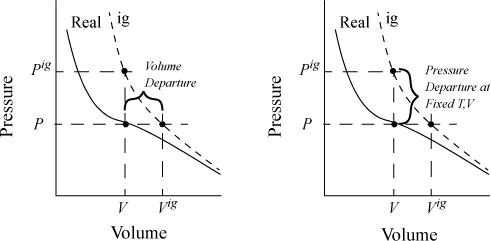
Figure 8.3. Comparison of real fluid and ideal gas isotherms at the same temperature, demonstrating the departure function, and the departure function at fixed T,V.
To calculate the change in internal energy along an isotherm for the real fluid, we write:

![]() The departure for property M is at fixed T and, P and is given by (M–Mig). The departure at fixed T,V is also useful (particularly in Chapter 15) and is denoted by (M–Mig)TV.
The departure for property M is at fixed T and, P and is given by (M–Mig). The departure at fixed T,V is also useful (particularly in Chapter 15) and is denoted by (M–Mig)TV.
For an ideal gas:
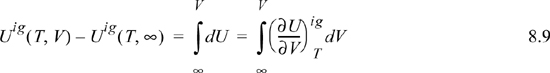
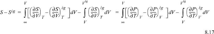
Since the real fluid approaches the ideal gas at infinite volume, we may take the difference in these two equations to find the departure function at fixed T,V,

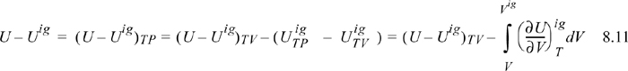
where (U – Uig)T, V = ∞ drops out because the real fluid energy approaches the ideal gas at infinite volume (low pressure). We have obtained a calculation with the real fluid in our desired state (T,P,V); however, we are referencing an ideal gas at the same volume rather than the same pressure. To see the difference, consider methane at 250 K, 10 MPa, and 139 cm3/mole. The volume of the ideal gas should be Vig = 8.314·250/10 = 208 cm3/mole. To obtain the departure function denoted by (U – Uig) (which is referenced to an ideal gas at the same pressure), we must add a correction to change the ideal gas state to match the pressure rather than the volume. Note in Fig. 8.3 that the real state is the same for both departure functions—the difference between the two departure functions has to do with the volume used for the ideal gas part of the calculation. The result is
We have already solved for (∂Uig/∂V)T (see Example 6.6 on page 238), and found that it is equal to zero. We are fortunate in this case because the internal energy of an ideal gas does not depend on the volume. When it comes to properties involving entropy, however, the dependency on volume requires careful analysis. Then the systematic treatment developed above is quite valuable.
Making these substitutions, we have

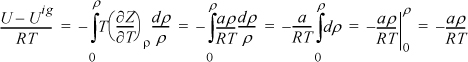
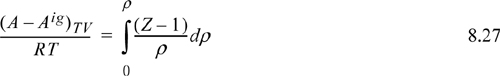
If we transform the integral to density, the resultant expression is easier to integrate for a cubic equation of state. Recognizing dV = –dρ/ρ2, and as V → ∞, ρ → 0, thus,

The above equation applies the chain rule in a way that may not be obvious at first:
We now have a compact equation to apply to any equation of state. Knowing Z = Z(T, ρ), (e.g., Eqn. 7.15, the Peng-Robinson model), we simply differentiate once, cancel some terms, and integrate. This a perfect sample application of the multivariable calculus that should be familiar at this stage in the curriculum. More importantly, we have developed a systematic approach to solving for any departure function. The steps for a system where Z = Z(T, ρ) are as follows.
1. Write the derivative of the property with respect to volume at constant T. Convert to derivatives of measurable properties using methods from Chapter 6.
2. Write the difference between the derivative real fluid and the derivative ideal gas.
3. Insert integral over dV and limits from infinite volume (where the real fluid and the ideal gas are the same) to the system volume V.
4. Add the necessary correction integral for the ideal gas from V to Vig. (This will be more obvious for entropy.)
5. Transform derivatives to derivatives of Z. Evaluate the derivatives symbolically using the equation of state and integrate analytically.
6. Rearrange in terms of density and compressibility factor to make it more compact.
Some of these steps could have been omitted for the internal energy, because (∂Uig/∂V)T = 0. Steps 1 through 4 are slightly different when Z = Z(T, P) such as with the truncated virial EOS. To see the importance of all the steps, consider the entropy departure function.
Example 8.1. Internal energy departure from the van der Waals equation
Derive the internal energy departure function for the van der Waals equation. Suppose methane is compressed from 200 K and 0.1 MPa to 220 K and 60 MPa. Which is the larger contribution in magnitude to ΔU, the ideal gas contribution or the departure function? Use CP from the back flap and ignore temperature dependence.
Solution
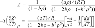
For methane, a = 230030 J-cm3/mol2 and b = 43.07 cm3/mol were calculated by the critical point criteria in Example 7.7 on page 271. Deriving the departure function, –T(dZ/dT)ρ = –aρ/RT, because the repulsive part is constant with respect to T. Substituting,
Because Tr > 1 there is only one real root. A quick but crude computation of ρ is to rearrange as Zbρ = bP/RT = bρ/(1 – bρ) – (a/bRT)(bρ)2.
At state 2, 220 K and 60 MPa,
60·43.07/(8.314·220) = bρ/(1 – bρ) – 230030/(43.07·8.314·220)(bρ)2.
Taking an initial guess of bρ = 0.99 and solving iteratively gives bρ = 0.7546, so
(U2 – U2ig)/RT = –230030·0.7546/(43.07·8.314·220) = –2.203.
At state 1, 200 K and 0.1 MPa,
0.1·43.07/(8.314·200) = bρ/(1 – bρ) – 230030/(43.07·8.314·200)(bρ)2.
Taking an initial guess of bρ = 0.99 and solving iteratively gives bρ = 0.00290, so
(U1 – U1ig)/RT = –230030·0.00290/(43.07·8.314·200) = –0.00931.
ΔU = –2.203(8.314)220 + (4.3 – 1)·8.314(220 – 200) + 0.00931(8.314)200 = –4030 + 549 + 15 = –3466 J/mol. The ideal gas part (549) is 14% as large in magnitude as the State 2 departure function (–4030) for this calculation. Clearly, State 2 is not an ideal gas.
Note that we do not need to repeat the integral for every new problem. For the van der Waals equation, the formula (U–Uig)/(RT) = –(aρ)/(RT) may readily be used whenever the van der Waals fluid density is known for a given temperature.
8.3. Entropy Departure Function
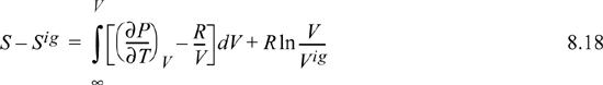
To calculate the entropy departure, adapt Eqn. 8.11,

Inserting the integral for the departure at fixed {T, V}, we have (using a Maxwell relation),
Since ![]() , we may readily integrate the ideal gas integral (note that this is not zero whereas the analogous equation for energy was zero):
, we may readily integrate the ideal gas integral (note that this is not zero whereas the analogous equation for energy was zero):
Recognizing Vig = RT/P, V/Vig = PV/RT = Z,
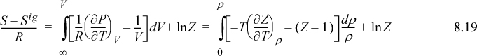
where Eqn. 8.15 has been applied to the relation for the partial derivative of P.
Note the ln(Z) term on the end of this equation. It arises from the change in ideal gas ![]() represented by the integral in Eqn. 8.16. Changes in states like this may seem pedantic and arcane, but they turn out to be subtle details that often make a big difference numerically. In Example 7.4 on page 266, we determined vapor and liquid roots for Z. The vapor root was close to unity, so ln(Z) would make little difference in that case. For the liquid root, however, Z = 0.016, and ln(Z) makes a substantial difference. These arcane details surrounding the subject of state specification are the thermodynamicist’s curse.
represented by the integral in Eqn. 8.16. Changes in states like this may seem pedantic and arcane, but they turn out to be subtle details that often make a big difference numerically. In Example 7.4 on page 266, we determined vapor and liquid roots for Z. The vapor root was close to unity, so ln(Z) would make little difference in that case. For the liquid root, however, Z = 0.016, and ln(Z) makes a substantial difference. These arcane details surrounding the subject of state specification are the thermodynamicist’s curse.
8.4. Other Departure Functions
The remainder of the departure functions may be derived from the first two and the definitions,

![]() The departures for U and S are the building blocks from which the other departures can be written by combining the relations derived in the previous sections.
The departures for U and S are the building blocks from which the other departures can be written by combining the relations derived in the previous sections.
where we have used PVig = RT for the ideal gas in the enthalpy departure. Using H – Hig just derived,
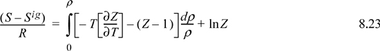
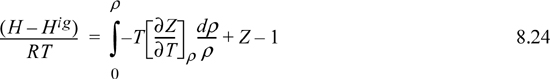
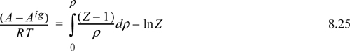
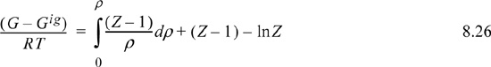
8.5. Summary of Density-Dependent Formulas
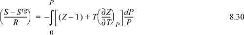
Formulas for departures at fixed T,P are listed below. These formulas are useful for an equation of state written most simply as Z = f(T,ρ) such as cubic EOSs. For treating cases where an equation of state is written most simply as Z = f (T,P) such as the truncated virial EOS, see Section 8.6.
Useful formulas at fixed T,V include:

8.6. Pressure-Dependent Formulas
Occasionally, our equation of state is difficult to integrate to obtain departure functions using the formulas from Section 8.5. This is because the equation of state is more easily arranged and integrated in the form Z = f (T,P), such as the truncated virial EOS. For treating cases where an equation of state is written most simply as Z = f(T,ρ) such as a cubic EOS, see Section 8.5. We adapt the procedures given earlier in Section 8.2.
1. Write the derivative of the property with respect to pressure at constant T. Convert to derivatives of measurable properties using methods from Chapter 6.
2. Write the difference between the derivative real fluid and the derivative ideal gas.
3. Insert integral over dP and limits from P = 0 (where the real fluid and the ideal gas are the same) to the system pressure P.
4. Transform derivatives to derivatives of Z. Evaluate the derivatives symbolically using the equation of state and integrate analytically.
5. Rearrange in terms of density and compressibility factor to make it more compact.
We omit derivations and leave them as a homework problem. The two most important departure functions at fixed T,P are
The other departure functions can be derived from these using Eqns. 8.20 and 8.21. Note the mathematical similarity between P in the pressure-dependent formulas and ρ in the density-dependent formulas.
8.7. Implementation of Departure Formulas
The tasks that remain are to select a particular equation of state, take the appropriate derivatives, make the substitutions, develop compact expressions, and add up the change in properties. The good news is that many years of engineering research have yielded several preferred equations of state (see Appendix D) which can be applied generally to any application with a reasonable degree of accuracy. For the purposes of the text, we use the Peng-Robinson equation or virial equation to illustrate the principles of calculating properties. However, many applications require higher accuracy; new equations of state are being developed all the time. This means that it is necessary for each student to know how to adapt the departure function method to new situations as they come along.
The following example illustrates the procedure with an equation of state that is sufficiently simple that it can be applied with either the density-dependent formulas or the pressure-dependent formulas. Although the intermediate steps are a little different, the final answer is the same, of course.
Example 8.2. Real entropy in a combustion engine
A properly operating internal combustion engine requires a spark plug. The cycle involves adiabatically compressing the fuel-air mixture and then introducing the spark. Assume that the fuel-air mixture in an engine enters the cylinder at 0.08 MPa and 20°C and is adiabatically and reversibly compressed in the closed cylinder until its volume is 1/7 the initial volume. Assuming that no ignition has occurred at this point, determine the final T and P, as well as the work needed to compress each mole of air-fuel mixture. You may assume that ![]() for the mixture is 32 J/mole-K (independent of T), and that the gas obeys the equation of state,
for the mixture is 32 J/mole-K (independent of T), and that the gas obeys the equation of state,
PV = RT + aP
where a is a constant with value a = 187 cm3/mole. Do not assume that CV is independent of ρ. Solve using density integrals.
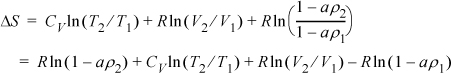
The system is taken as a closed system of the gas within the piston/cylinder. Because there is no flow, the system is irreversible, and reversible, the entropy balance becomes
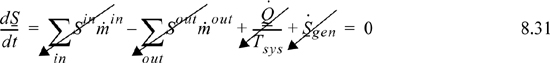
showing that the process is isentropic. To find the final T and P, we use the initial state to find the initial entropy and molar volume. Then at the final state, the entropy and molar volume are used to determine the final T and P.
This example helps us to understand the difference between departure functions at fixed T and V and departure functions at fixed T and P. The equation of state in this case is simple enough that it can be applied either way. It is valuable to note how the ln(Z) term works out. Fixed T and V is convenient since the volume change is specified in this example, and we cover this as Method I, and then use fixed T and P as Method II.
This EOS is easy to evaluate with either the pressure integrals of Section 8.6 or the density integrals of Section 8.5. The problem statement asks us to use density integrals.a First, we need to rearrange our equation of state in terms of Z = f (T, ρ). This rearrangement may not be immediately obvious. Note that dividing all terms by RT gives PV/RT = 1 + aP/RT. Note that Vρ = 1. Multiplying the last term by Vρ, Z = 1 + aZρ which rearranges to
Also, we find the density at the two states using the equation of state,
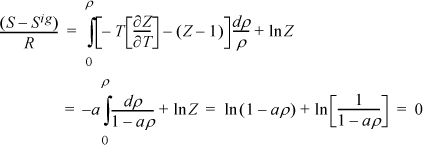
Method I. In terms of fixed T and V, ![]() ;
; ![]()

Method II. In terms of T and P,
Since the departure is zero, it drops out of the calculations.
![]() . However, since we are given the final volume, we need to calculate the final pressure. Note that we cannot insert the ideal gas law into the pressure ratio in the last term even though we are performing an ideal gas calculation; we must use the pressure ratio for the real gas.
. However, since we are given the final volume, we need to calculate the final pressure. Note that we cannot insert the ideal gas law into the pressure ratio in the last term even though we are performing an ideal gas calculation; we must use the pressure ratio for the real gas.
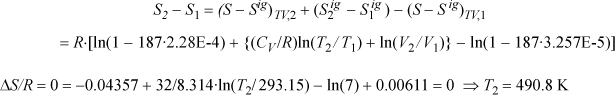
Now, if we rearrange, we can show that the result is the same as Method I:
This is equivalent to the equation obtained by Method I and T2 = 490.8 K.
Finally, ![]()
W = ΔU = (U – Uig)2 + CVΔT –(U – Uig)1 = 0 + CVΔT – 0 = 6325 J/mole
a. The solution to the problem using pressure integrals is left as homework problem 8.7.
Examples 8.1 and 8.2 illustrate the procedures for deriving and computing the impacts of departure functions, but the equations are too simple to merit broad application. The generalized virial equation helps to broaden the coverage of compound types while retaining a simple functional form.
Example 8.3. Compression of methane using the virial equation
Methane gas undergoes a continuous throttling process from upstream conditions of 40°C and 20 bars to a downstream pressure of 1 bar. What is the gas temperature on the downstream side of the throttling device? An expression for the molar ideal gas heat capacity of methane is CP = 19.25 + 0.0523 T + 1.197E-5 T2–1.132E-8 T3; T [≡] K; CP [≡] J/mol–K
The virial equation of state (Eqns. 7.6–7.10) may be used at these conditions for methane:
Z = 1 + BP/RT = 1 + (B0 + ωB1)Pr/Tr
where B0 = 0.083 – 0.422/Tr1.6 and B1 = 0.139 – 0.172/Tr4.2
Solution
Since a throttling process is isenthalpic, the enthalpy departure will be used to calculate the outlet temperature.
ΔH = 0 = H2–H1 = (H2 – H2ig) + (H2ig – H1ig) – (H1 – H1ig)
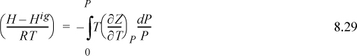
The enthalpy departure for the first and third terms in parentheses on the right-hand side can be calculated using Eqn. 8.29. Because Z(P,T), we use Eqn. 8.29. For the integrand, the temperature derivative of Z is required. Recognizing B is a function of temperature only and differentiating,
Inserting the derivative into Eqn 8.29,
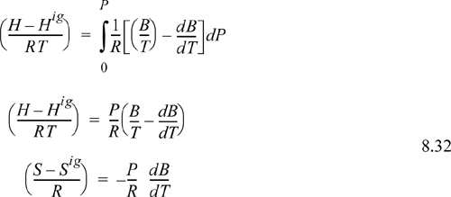
We can easily show by differentiating Eqns. 7.8 and 7.9,

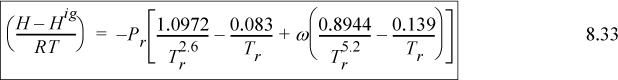
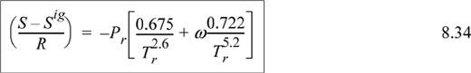
Substituting the relations for B0, B1, dB0/dTr and dB1dTr into Eqn. 8.32 for the departure functions for a pure fluid, we get
Assuming a small temperature drop, the heat capacity will be approximately constant over the interval, CP ≈ 36 J/mole-K.
For a throttle, ΔH = 0 ⇒ (H – Hig)2 + 36(T2 – 40) + 287 = 0.
Trial and error at state 2 where P = 1 bar, T2 = 35°C ⇒ –13 + 36(35 – 40) + 287 = 94.
T2 = 30°C ⇒ –13 + 36(30 – 40) + 287 = –87
Interpolating, T2 = 35 + (35 – 30)/(94 + 87)(–94) = 32.4°C, another trial would show this is close.
Finally, the Peng-Robinson model is sufficiently sophisticated to permit broad application, but the derivations are quite tedious. It may be helpful to see how simple the eventual computations are before getting overwhelmed with the mathematics. Hence, the first example below simply shows how to obtain results based on the computer programs furnished with the text. The subsequent examples confront the derivation of the departure function formulas that appear in the computer programs for the Peng-Robinson equation.
Example 8.4. Computing enthalpy and entropy departures from the Peng-Robinson equation
Propane gas undergoes a change of state from an initial condition of 5 bar and 105°C to 25 bar and 190°C. Compute the change in enthalpy and entropy.
Solution
For propane, Tc = 369.8 K; Pc = 4.249 MPa; ω = 0.152. The heat capacity coefficients are given by A = –4.224, B = 0.3063, C = –1.586E-4, D = 3.215E-8. We may use the spreadsheet Preos.xlsx or PreosPropsMenu.m. If we select the spreadsheet, we can use the PROPS page to calculate thermodynamic properties. Using the m-file, we specify the species ID number in the function call to PreosPropsMenu.m and find the departures in the command window. We extract the following results:
For State 2:
For State 1:
Ignoring the specification of the reference state for now (refer to Example 8.8 on page 320 to see how to apply the reference state approach), divide the solution into the three stages described in Section 8.1: I. departure Function; II. ideal gas; III. departure function.
The overall solution path for H2 – H1 is
Similarly, for S2 – S1 =
The three steps that make up the overall solution are covered individually.
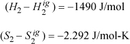
Step I. Departures at state 2 from the spreadsheet:
Step II. State change for ideal gas: The ideal gas enthalpy change has been calculated in Example 2.5 on page 60.
The ideal gas entropy has been calculated in Example 4.6 on page 151:
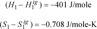
Step III. Departures at state 1 from the spreadsheet:
The total changes may be obtained by summing the steps of the calculation.
ΔH = –1490 + 8405 + 401 = 7316 J/mole
ΔS = –2.292 + 6.613 + 0.708 = 5.029 J/mole-K
We have laid the foundation for deriving and applying departure functions given an equation of state. What remains is to organize our efforts to enable convenient and accurate calculations for the myriad of applications that we may encounter. Since these types of computations must be repeated many times, it is worthwhile to implement a broadly applicable (“one size fits all”) thermodynamic model and construct a computer program that facilitates input and output. The derivations and programming are more tedious, but they repay the invested effort through multiple applications. The examples below illustrate the derivations for the Peng-Robinson model, but several alternative models could have formed the basis for broad application. You should be able to demonstrate your mastery of the model equations underlying the programming by performing equivalent derivations with alternative models like those illustrated in the homework problems
Example 8.5. Enthalpy departure for the Peng-Robinson equation
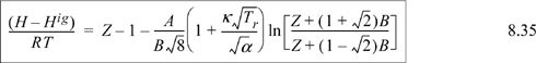
Obtain a general expression for the enthalpy departure function of the Peng-Robinson equation.
Solution
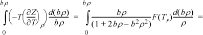
Since the Peng-Robinson equation is of the form Z(T,ρ), we can only solve with density integrals.
where da/dT is given in Eqn. 7.18. Inserting,
We introduce F(Tr) as a shorthand.
Also, B ≡ bP/RT ⇒ bρ = B/Z and A ≡ aP/R2T2 ⇒ a/bRT = A/B. Note that the integration is simplified by integration over bρ (see Eqn. B.34).
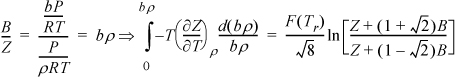

Example 8.6. Gibbs departure for the Peng-Robinson equation
Obtain a general expression for the Gibbs energy departure function of the Peng-Robinson equation.
Solution
The answer is obtained by evaluating Eqn. 8.26. The argument for the integrand is
Evaluating the integral (similar to the integral in Example 8.5), noting again the change in integration variables,

Making the result dimensionless,

It is often valuable to recognize simplifications that may circumvent the tedium. If two models are similar, you can reuse the part of the derivation that is equivalent. If thermodynamic identities can be used to substitute major portions of a derivation, so much the better. Productive engineers should be aware of opportunities to leverage their time efficiently, as illustrated below.
Example 8.7. U and S departure for the Peng-Robinson equation
Derive the departure functions for internal energy and entropy of the Peng-Robinson equation. Hint: You could start with Eqns. 8.22 and 8.23, or you could use the results of Examples 8.5 and 8.6 without further integration as suggested by Eqn. 8.20 and Eqn. 8.21.
Solution
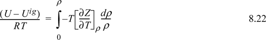
By Eqn. 8.20, the U departure can be obtained by dropping the “Z – 1” term from Eqn. 8.35. We may immediately write:

By Eqn. 8.21, the entropy departure can be obtained by the difference between the enthalpy departure and Gibbs energy departure, available in Eqns. 8.35 and 8.36. Then, we may immediately write
8.8. Reference States
If we wish to calculate state changes in a property, then the reference state is not important, and all reference state information drops out of the calculation. However, if we wish to generate a chart or table of thermodynamic properties, or compare our calculations to a thermodynamic table/chart, then designation of a reference state becomes essential. Also, if we need to solve unsteady-state problems, the reference state is important because the answer may depend on the reference state as shown in Example 2.15 on page 81. The quantity HR – UR = (PV)R is non-zero, and although we may substitute (PV)R = RTR for an ideal gas, for a real fluid we must use (PV)R = ZRRTR, where ZR has been determined at the reference state. We also may use a real fluid reference state or an ideal gas reference state. Whenever we compare our calculations with a thermodynamic chart/table, we must take into consideration any differences between our reference state and that of the chart/table. Therefore, to specify a reference state for a real fluid, we need to specify:
Pressure
Temperature
In addition we must specify the state of aggregation at the reference state from one of the following:
1. Ideal gas
2. Real gas
3. Liquid
4. Solid
Further, we set SR = 0, and either (but not both) of UR and HR to zero. The principle of using a reference state is shown in Fig. 8.4 and is similar to the calculation outlined in Fig. 8.2 on page 303.

Figure 8.4. Illustration of calculation of state changes for a generic property M using departure functions where M is U, H, S, G, or A. The calculations are an extension of the principles used in Fig. 8.2 where the initial state is designated as the reference state.
Ideal Gas Reference States
For an ideal gas reference state, to calculate a value for enthalpy, we have

where the quantity in parentheses is the departure function from Section 8.5 or 8.6 and ![]() may be set to zero. An analogous equation may be written for the internal energy. Because entropy of the ideal gas depends on pressure, we must include a pressure integral for the ideal gas,
may be set to zero. An analogous equation may be written for the internal energy. Because entropy of the ideal gas depends on pressure, we must include a pressure integral for the ideal gas,
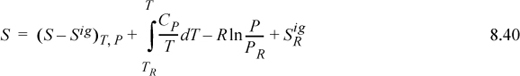
where the reference state value, ![]() , may be set to zero. From these results we may calculate other properties using relations from Section 6.1: G = H – TS, A = U – TS, and U = H – PV.
, may be set to zero. From these results we may calculate other properties using relations from Section 6.1: G = H – TS, A = U – TS, and U = H – PV.
Real Fluid Reference State
For a real fluid reference state, to calculate a value for enthalpy, we adapt the procedure of Eqn. 8.5:

For entropy:

Changes in State Properties
Changes in state properties are independent of the reference state, or reference state method. To calculate changes in enthalpy, we have the analogy of Eqn. 8.5:

To calculate entropy changes:

Example 8.8. Enthalpy and entropy from the Peng-Robinson equation
Propane gas undergoes a change of state from an initial condition of 5 bar and 105°C to 25 bar and 190°C. Compute the change in enthalpy and entropy. What fraction of the total change is due to the departure functions at 190°C? The departures have been used in Example 8.4, but now we can use the property values directly.
Solution
For propane, Tc = 369.8 K; Pc = 4.249 MPa; and ω = 0.152. The heat capacity coefficients are given by A = –4.224, B = 0.3063, C = –1.586E-4, and D = 3.215E-8. For Preos.xlsx, we can use the “Props” page to specify the critical constants and heat capacity constants. The reference state is specified on the companion spreadsheet “Ref State.” An arbitrary choice for the reference state is the liquid at 230 K and 0.1 MPa. Returning to the PROPS worksheet and specifying the desired temperature and pressure gives the thermodynamic properties for V,U,H, and S.
The changes in the thermodynamic properties are ΔH = 7315J/mole and ΔS = 5.024J/mole-K, identical to the more tediously determined values of Example 8.4 on page 314. The purpose of computing the fractional change due to departure functions is to show that we understand the roles of the departure functions and how they fit into the overall calculation. For the enthalpy, the appropriate fraction of the total change is 20%, for the entropy, 46%.
Example 8.9. Liquefaction revisited
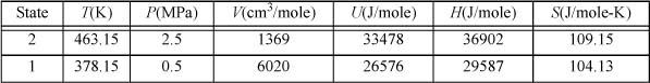
Reevaluate the liquefaction of methane considered in Example 5.5 on page 213 utilizing the Peng-Robinson equation. Previously the methane chart was used. Natural gas, assumed here to be pure methane, is liquefied in a simple Linde process. The process is summarized in Fig. 8.5. Compression is to 60 bar, and precooling is to 300 K. The separator is maintained at a pressure of 1.013 bar and unliquefied gas at this pressure leaves the heat exchanger at 295 K. What fraction of the methane entering the heat exchanger is liquefied in the process?
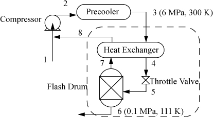
Figure 8.5. Linde liquefaction schematic.
Before we calculate the enthalpies of the streams, a reference state must be chosen. The reference state is arbitrary. Occasionally, an energy balance is easier to solve by setting one of the enthalpies to zero by selecting a stream condition as the reference state. To illustrate the results let us select a reference state of H = 0 at the real fluid at the state of Stream 3 (6 MPa and 300 K). Because state 3 is the reference state, the H3 = 0. The results of the calculations from the Peng-Robinson equation are summarized in Fig. 8.6.
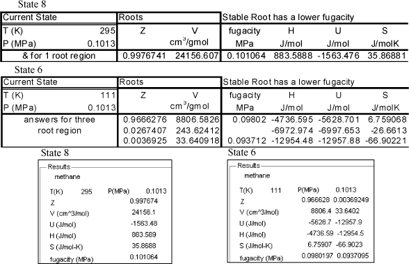
Figure 8.6. Summary of enthalpy calculations for methane as taken from the files Preos.xlsx (above) and PreosPropsMenu.m below.
The fraction liquefied is calculated by the energy balance: m3H3 = m8H8 + m6H6; then incorporating the mass balance: H3 = (1 – m6/m3)H8 + (m6/m3)H6.
The throttle valve is isenthalpic (see Section 2.13). The flash drum serves to disengage the liquid and vapor exiting the throttle valve. The fraction liquefied is (1 – q) = m6/m3 = (H3 – H8)/(H6 – H8) = (0 – 883)/(–12,954 – 883) = 0.064, or 6.4% liquefied. This is in good agreement with the value obtained in Example 5.5 on page 213.
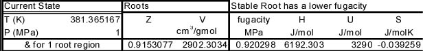
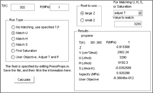
Example 8.10. Adiabatically filling a tank with propane
Propane is available from a reservoir at 350 K and 1 MPa. An evacuated cylinder is attached to the reservoir manifold, and the cylinder is filled adiabatically until the pressure is 1 MPa. What is the final temperature in the cylinder?
Solution
The critical properties, acentric factor and heat capacity constants, are entered on the “Props” page of Preos.xlsx. On the “Ref State” page, the reference state is arbitrarily selected as the real vapor at 298 K and 0.1 MPa, and HR = 0. At the reservoir condition, propane is in the one-root region with Z = 0.888, H = 3290 J/mol, U = 705 J/mol, and S = –7.9766 J/mol-K. The same type of problem has been solved for an ideal gas in Example 2.16 on page 82; however, in this example the ideal gas law cannot be used. The energy balance reduces to Uf = Hin, where Hin = 3290 J/mol. In Excel, the answer is easily found by using Solver to adjust the temperature on the “Props” page until U = 3290 J/mol. The converged answer is 381 K. In MATLAB, the dialog boxes can be used to match U = 3290 J/mol by adjusting T. In the MATLAB window, note that the final T is shown in the “Results” box. The initial guess is preserved in the upper left.
8.9. Generalized Charts for the Enthalpy Departure
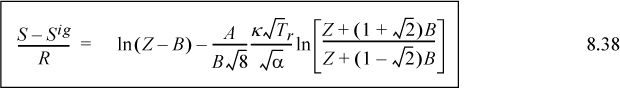
As in the case of the compressibility factor, it is often useful to have a visual idea of how generalized properties behave. Fig. 8.7 on page 324 is analogous to the compressibility factor charts from the previous chapter except that the formula for enthalpy is (H – Hig) = (H – Hig)0 + ω(H – Hig)1. Note that one primary influence in determining the liquid enthalpy departure is the heat of vaporization. Also, the subcritical isotherms shift to liquid behavior at lower pressures when the saturation pressures are lower. The enthalpy departure function is somewhat simpler than the compressibility factor in that the isotherms do not cross one another. Note that the temperature used to make the departure dimensionless is Tc. A sample calculation for propane at 463.15 K and 2.5 MPa gives Hig – H = [0.45 + 0.152(0.2)] (8.314) 369.8 = 1480 J/mole compared to 1489.2 from the Peng-Robinson equation.
8.10. Summary
The study of departure functions often causes students great difficulty. That is understandable since it involves simultaneous application of physics and multivariable calculus. This may be the first instance in which students have applied these subjects in combination to such an extent. On the other hand, it is impressive to see what can be accomplished with these tools: the functional equivalent of “steam tables” for any compound in the universe (given a reliable equation of state).
When you get beyond the technical details, however, it seems obvious that there is a difference between an ideal gas and a real fluid. As the accountants for energy movements, we need to be able to account for such contributions. Our method is to first add up all the contributions as if everything behaved like an ideal gas, then to compute and add up all the departures from ideal gas behavior. We apply this over and over again. The calculations are greatly facilitated by computers such that the minimum requirement is the knowledge of what calculation is required and which buttons to push. The purpose of this chapter was to turn your attention to developing a better understanding of the subtleties underlying the equations inside the computer programs.
Your understanding of departure functions is reflected in your ability to develop expressions for various equations of state, as well as the mechanics of adding up the numerical quantities. We covered several derivations, especially for the Peng-Robinson model, and you should be able to reproduce that procedure for other models. Obtaining numerical results occasionally requires iteration and careful consideration of the key constraints. For example, an isentropic compression may transition from the three-root region to the one-root region and your awareness of issues like this corresponds directly with your understanding of how the calculations are performed. Try to rewrite the Excel files yourself, to ensure that you fully comprehend them.
Important Equations
Eqns. 8.22–8.30 stand out in this chapter as the starting point for deriving the necessary departure function expressions for any equation of state. It is tempting to use spreadsheets or programs to add up the contributions from departure functions, reference states, and ideal gas temperature effects mindlessly, like a human computer. But keep in mind that a major goal is to teach the development of model equations, as well as their application. Your skill in developing model equations for novel applications can transcend the study of thermodynamics. Master the derivations behind the programs as well as the mechanics of implementing them.

Figure 8.7. Generalized charts for estimating (H – Hig)/RTc using the Lee-Kesler equation of state. (H – Hig)0/RTc uses ω = 0.0, and (H – Hig)1/RTc is the correction factor for a hypothetical compound with ω = 1.0. Divide by reduced temperature to obtain the enthalpy departure function.
8.11. Practice Problems
P8.1. Develop an expression for the Gibbs energy departure function based on the Redlich-Kwong (1958) equation of state:
(ANS. (G – Gig)/RT = –ln(1 – bρ) – aln(1 + bρ)/(bRT3/2) + Z – 1 – lnZ)
P8.2. For certain fluids, the equation of state is given by Z = 1 – bρ/Tr.
Develop an expression for the enthalpy departure function for fluids of this type. (ANS. –2bρ/Tr)
P8.3. In our discussion of departure functions we derived Eqn. 8.14 for the internal energy departure for any equation of state.
a. Derive the analogous expression for ![]() .
.
b. Derive an expression for ![]() in terms of a, b, ρ, and T for the equation of state:
in terms of a, b, ρ, and T for the equation of state:
P8.4. Even in the days of van der Waals, the second virial coefficient for square-well fluids (λ = 1.5) was known to be B/b = 4 + 9.5 [exp(NAε/RT) – 1]. Noting that ex ~ 1 + x + x2/2 + ..., this observation suggests the following equation of state:
Derive an expression for the Helmholtz energy departure function for this equation of state. (ANS. –4ln(1 – bρ) – 9.5NAεbρ/kT)
P8.5. Making use of the Peng-Robinson equation, calculate ΔH, ΔS, ΔU, and ΔV for 1 gmol of 1,3-butadiene when it is compressed from 25 bar and 400 K to 125 bar and 550 K. (ANS. ΔH = 12,570 J/mol; ΔS = 17.998 J/mol-K; ΔU = 11,690 J/mol; ΔV = –640.8 cm3/mol)
P8.6. Ethane at 425 K and 100 bar initially is contained in a 1 m3 cylinder. An adiabatic, reversible turbine is connected to the outlet of the tank and exhausted to atmosphere at 1 bar absolute.
a. Estimate the temperature of the first gas to flow out of the turbine. (ANS. 185 K)
b. Estimate the rate of work per mole at the beginning of this operation. (ANS. 8880 J/mol)
P8.7. Ethylene at 350°C and 50 bar is passed through an adiabatic expander to obtain work and exits at 2 bar. If the expander has an efficiency of 80%, how much work is obtained per mole of ethylene, and what is the final temperature of the ethylene? How does the final temperature compare with what would be expected from a reversible expander? (ANS. 11 kJ/mole, 450 K versus 404 K)
P8.8. A Rankine cycle is to operate on methanol. The boiler operates at 200°C (Psat = 4.087 MPa), and a superheater further heats the vapor. The turbine outlet is saturated vapor at 0.1027 MPa, and the condenser outlet is saturated liquid at 65°C (Psat = 0.1027 MPa). What is the maximum possible value for the cycle thermal efficiency (ηθ = –W/QH)? (ANS. 26%)
P8.9. An ordinary vapor-compression cycle is to be designed for superconductor application using N2 as refrigerant. The expansion is to 1 bar. A heat sink is available at 105 K. A 5 K approach should be sufficient. Roughly 100 Btu/hr must be removed. Compute the coefficient of performance (COP) and compare to the Carnot COP. Also, estimate the compressor’s power requirement (hp) assuming it is adiabatic and reversible. (ANS. 1.33, 0.3)
P8.10. Suppose ethane was compressed adiabatically in a 70% efficient continuous compressor. The downstream pressure is specified to be 1500 psia at a temperature not to exceed 350°F. What is the highest that the upstream temperature could be if the upstream pressure is 200 psia? (Hint: Neglect the upstream departure function.) (ANS. 269 K)
P8.11. As part of a liquefaction process, ammonia is throttled to 80% quality at 1 bar. If the upstream pressure is 100 bar, what must be the upstream temperature?
P8.12. An alternative to the pressure equation route from the molecular scale to the macroscopic scale is through the energy equation (Eqn. 7.51). The treatment is similar to the analysis for the pressure equation, but the expression for the radial distribution function must now be integrated over the range of the potential function.
a. Suppose that u(r) is given by the square-well potential (R = 1.5) and g(r) = 10 – 5(r/σ) for r > σ. Evaluate the internal energy departure function where ρσ3 = 1 and ε/kT = 1. (ANS. –5.7π)
b. Suppose that the radial distribution function at intermediate densities can be reasonably represented by: g ~ (1 + 2(σ/r)2) at all temperatures. Derive an expression for the attractive contribution to the compressibility factor for fluids that can be accurately represented by the Sutherland potential. (ANS. 3πρNAσ3NAε/RT)
8.12. Homework Problems
8.1. What forms does the derivative (∂CV/∂V)T have for a van der Waals gas and a Redlich-Kwong gas? (The Redlich-Kwong equation is given in Problem P8.1.) Comment on the results.
8.2. Estimate CP, CV, and the difference CP – CV in (J/mol-K) for liquid n-butane from the following data.2

8.3. Estimate CP, CV, and the difference CP – CV in (J/mol-K) for saturated n-butane liquid at 298 K n-butane as predicted by the Peng-Robinson equation of state. Repeat for saturated vapor.
8.4. Derive the integrals necessary for departure functions for U, G, and A for an equation of state written in terms of Z = f(T,P) using the integrals provided for H and S in Section 8.6.
a. Derive the enthalpy and entropy departure functions for a van der Waals fluid.
b. Derive the formula for the Gibbs energy departure.
8.6. The Soave-Redlich-Kwong equation is presented in problem 7.15. Derive expressions for the enthalpy and entropy departure functions in terms of this equation of state.
8.7. In Example 8.2 we wrote the equation of state in terms of Z = f (T,ρ). The equation of state is also easy to rearrange in the form Z = f (T,P). Rearrange the equation in this form, and apply the formulas from Section 8.6 to resolve the problem using departures at fixed T and P.
8.8. The ESD equation is presented in problem 7.19. Derive expressions for the enthalpy and entropy departure functions in terms of this equation of state.
8.9. A gas has a constant-pressure ideal-gas heat capacity of 15R. The gas follows the equation of state,
over the range of interest, where a = –1000 cm3/mole.
a. Show that the enthalpy departure is of the following form:
b. Evaluate the enthalpy change for the gas as it undergoes the state change:
T1 = 300 K, P1 = 0.1 MPa, T2 = 400 K, P2 = 2 MPa
8.10. Derive the integrated formula for the Helmholtz energy departure for the virial equation (Eqn. 7.7), where B is dependent on temperature only. Express your answer in terms of B and its temperature derivative.
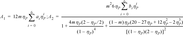
8.11. Recent research suggests the following equation of state, known as the PC-SAFT model.
a. Derive an expression for Z.
b. Derive the departure function for (U-Uig).
Note: ηP = bρ; m = constant proportional to molecular weight; ai, bi are constants.

8.12. Recent research in thermodynamic perturbation theory suggests the following equation of state.
a. Derive the departure function for (A – Aig)T,V.
b. Derive the departure function for (U – Uig).
Hint: substitute u = 0.7 + Texp(10ηP); ηP = bρ.
8.13. A gas is to be compressed in a steady-state flow reversible isothermal compressor. The inlet is to be 300 K and 1 MPa and the gas is compressed to 20 MPa. Assume that the gas can be modeled with equation of state
where a = 385.2 cm3-K/mol and b = 15.23 cm3/mol. Calculate the required work per mole of gas.
8.14. A 1 m3 isolated chamber with rigid walls is divided into two compartments of equal volume. The partition permits transfer of heat. One side contains a nonideal gas at 5 MPa and 300 K and the other side contains a perfect vacuum. The partition is ruptured, and after sufficient time for the system to reach equilibrium, the temperature and pressure are uniform throughout the system. The objective of the problem statements below is to find the final T and P.
The gas follows the equation of state
where b = 20 cm3/mole; a = 40,000 cm3K/mole; and CP = 41.84 + 0.084T(K) J/mol-K.
a. Set up and simplify the energy balance and entropy balance for this problem.
b. Derive formulas for the departure functions required to solve the problem.
b. Determine the final P and T.
8.15. P-V-T behavior of a simple fluid is found to obey the equation of state given in problem 8.14.
a. Derive a formula for the enthalpy departure for the fluid.
b. Determine the enthalpy departure at 20 bar and 300 K.
c. What value does the entropy departure have at 20 bar and 300 K?
8.16. Using the Peng-Robinson equation, estimate the change in entropy (J/mole-K) for raising butane from a saturated liquid at 271 K and 1 bar to a vapor at 352 K and 10 bar. What fraction of this total change is given by the departure function at 271 K? What fraction of this change is given by the departure function at 352 K?
8.17. Suppose we would like to establish limits for the rule T2 = T1(P2/P1)R/CP by asserting that the estimated T2 should be within 5% of the one calculated using the departure functions. For ω = 0 and Tr = [1, 10] at state 1, determine the values of Pr where this assertion holds valid by using the Peng-Robinson equation as the benchmark.
8.18. A piston contains 2 moles of propane vapor at 425 K and 8.5 MPa. The piston is taken through several state changes along a pathway where the total work done by the gas is 2 kJ. The final state of the gas is 444 K and 3.4 MPa. What is the change, ΔH, for the gas predicted by the Peng-Robinson equation and how much heat is transferred? Note: A reference state is optional; if one is desired, use vapor at 400 K and 0.1 MPa.
8.19. N.B. Vargaftik3 (1975) lists the experimental values in the following table for the enthalpy departure of isobutane at 175°C. Compute theoretical values and their percent deviations from experiment by the following
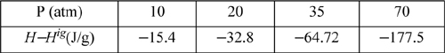
a. The generalized charts
b. The Peng-Robinson equation
8.20. n-pentane is to be heated from liquid at 298 K and 0.01013 MPa to vapor at 360 K and 0.3 MPa. Compute the change in enthalpy using the Peng-Robinson equation of state. If a reference state is desired, use vapor at 310 K, 0.103 MPa, and provide the enthalpy departure at the reference state.
8.21. For each of the fluid state changes below, perform the following calculations using the Peng-Robinson equation: (a) Prepare a table and summarize the molar volume, enthalpy, and entropy for the initial and final states; (b) calculate ΔH and ΔS for the process; and (c) compare with ΔH and ΔS for the fluid modeled as an ideal gas. Specify your reference states.
a. Propane vapor at 1 bar and 60°C is compressed to a state of 125 bar and 250°C.
b. Methane vapor at –40°C and 0.1013 MPa is compressed to a state of 10°C and 7 MPa.
8.22. 1 m3 of CO2 initially at 150°C and 50 bar is to be isothermally compressed in a frictionless piston/cylinder device to a final pressure of 300 bar. Calculate the volume of the compressed gas, ΔU, the work done to compress the gas, and the heat flow on compression assuming
a. CO2 is an ideal gas.
b. CO2 obeys the Peng-Robinson equation of state.
8.23. Solve problem 8.22 for an adiabatic compression.
8.24. Consider problem 3.11 using benzene as the fluid rather than air and eliminating the ideal gas assumption. Use the Peng-Robinson equation. For the same initial state,
a. The final tank temperature will not be 499.6 K. What will the temperature be?
b. What is the number of moles left in the tank at the end of the process?
b. Write and simplify the energy balance for the process. Determine the final temperature of the piston/cylinder gas.
8.25. Solve problem 8.24 using n-pentane.
8.26. A tank is divided into two equal halves by an internal diaphragm. One half contains argon at a pressure of 700 bar and a temperature of 298 K, and the other chamber is completely evacuated. Suddenly, the diaphragm bursts. Compute the final temperature and pressure of the gas in the tank after sufficient time has passed for equilibrium to be attained. Assume that there is no heat transfer between the tank and the gas, and that argon:
a. Is an ideal gas
b. Obeys the Peng-Robinson equation
8.27. The diaphragm of the preceding problem develops a small leak instead of bursting. If there is no heat transfer between the gas and tank, what is the temperature and pressure of the gas in each tank after the flow stops? Assume that argon obeys the Peng-Robinson equation.
8.28. A practical application closely related to the above problem is the use of a compressed fluid in a small can to reinflate a flat tire. Let’s refer to this product as “Fix-a-flat.” Suppose we wanted to design a fix-a-flat system based on propane. Let the can be 500 cm3 and the tire be 40,000 cm3. Assume the tire remains isothermal and at low enough pressure for the ideal gas approximation to be applicable. The can contains 250 g of saturated liquid propane at 298 K and 10 bar. If the pressure in the can drops to 0.85 MPa, what is the pressure in the tire and the amount of propane remaining in the can? Assuming that 20 psig is enough to drive the car for a while, is the pressure in the tire sufficient? Could another tire be filled with the same can?
8.29. Ethylene at 30 bar and 100°C passes through a throttling valve and heat exchanger and emerges at 20 bar and 150°C. Assuming that ethylene obeys the Peng-Robinson equation, compute the flow of heat into the heat exchanger per mole of ethylene.
8.30. In the final stage of a multistage, adiabatic compression, methane is to be compressed from –75°C and 2 MPa to 6 MPa. If the compressor is 76% efficient, how much work must be furnished per mole of methane, and what is the exit temperature? How does the exit temperature compare with that which would result from a reversible compressor? Use the Peng-Robinson equation.
a. Ethane at 280 K and 1 bar is continuously compressed to 310 K and 75 bar. Compute the change in enthalpy per mole of ethane using the Peng-Robinson equation.
b. Ethane is expanded through an adiabatic, reversible expander from 75 bar and 310 K to 1 bar. Estimate the temperature of the stream exiting the expander and the work per mole of ethane using the Peng-Robinson equation. (Hint: Is the exiting ethane vapor, liquid, or a little of each? The saturation temperature for ethane at 1 bar is 184.3 K.)
8.32. Our space program requires a portable engine to generate electricity for a space station. It is proposed to use sodium (Tc = 2300 K; Pc = 195 bar; ω = 0; CP/R = 2.5) as the working fluid in a customized form of a “Rankine” cycle. The high-temperature stream is not superheated before running through the turbine. Instead, the saturated vapor (T = 1444 K, Psat = 0.828 MPa) is run directly through the (100% efficient, adiabatic) turbine. The rest of the Rankine cycle is the usual. That is, the outlet stream from the turbine passes through a condenser where it is cooled to saturated liquid at 1155 K (this is the normal boiling temperature of sodium), which is pumped (neglect the pump work) back into the boiler.
a. Estimate the quality coming out of the turbine.
b. Compute the work output per unit of heat input to the cycle, and compare it to the value for a Carnot cycle operating between the same TH and TC.
8.33. Find the minimum shaft work (in kW) necessary to liquefy n-butane in a steady-state flow process at 0.1 MPa pressure. The saturation temperature at 0.1 MPa is 271.7 K. Butane is to enter at 12 mol/min and 0.1 MPa and 290 K and to leave at 0.1 MPa and 265 K. The surroundings are at 298 K and 0.1 MPa.
8.34. The enthalpy of normal liquids changes nearly linearly with temperature. Therefore, in a single-pass countercurrent heat exchanger for two normal liquids, the temperature profiles of both fluids are nearly linear. However, the enthalpy of a high-pressure gas can be nonlinearly related to temperature because the constant pressure heat capacity becomes very large in the vicinity of the critical point. For example, consider a countercurrent heat exchanger to cool a CO2 stream entering at 8.6 MPa and 115°C. The outlet is to be 8.6 MPa and 22°C. The cooling is to be performed using a countercurrent stream of water that enters at 10°C. Use a basis of l mol/min of CO2.
a. Plot the CO2 temperature (°C) on the ordinate versus H on the abscissa, using H = 0 for the outlet state as the reference state.
b. Since dHwater/dx = dHCO2/dx along a differential length, dx, of countercurrent of heat exchanger, the corresponding plot of T versus H for water (using the inlet state as the reference state) will show the water temperature profile for the stream that contacts the CO2. The water profile must remain below the CO2 profile for the water stream to be cooler than the CO2. If the water profile touches the CO2 profile, the location is known as a pinch point and the heat exchanger would need to be infinitely big. What is the maximum water outlet temperature that can be feasibly obtained for an infinitely sized heat exchanger?
c. Approximately what water outlet temperature should be used to ensure a minimum approach temperature for the two streams of approximately 10°C?
8.35. An alternative to the pressure equation route from the molecular scale to the macroscopic scale is through the energy equation (Eqn. 7.50). The treatment is similar to the analysis for the pressure equation, but the expression for the radial distribution function must now be integrated over the range of the potential function. Suppose that the radial distribution function can be reasonably represented by:
g = 0 for r < σ
g ~ 1 + ρNAσ6ε/(r3kT) for r > σ
at all temperatures and densities. Use Eqn. 7.50 to derive an expression for the internal energy departure function of fluids that can be accurately represented by the following:
a. The square-well potential with λsw = 1.5
b. The Sutherland potential
Evaluate each of the above expressions at ρNAσ3 = 0.6 and ε/kT = 1.
8.36. Starting with the pressure equation as shown in Chapter 6, evaluate the internal energy departure function at ρNAσ3 = 0.6 and ε/kT = 1 by performing the appropriate derivatives and integrations of the equation of state obtained by applying
g = 0 for r < σ
g ~ 1 + ρNAσ6ε/(r3kT) for r > σ
at all temperatures and densities:
a. The square-well potential with λsw = 1.5
b. The Sutherland potential
c. Compare these results to those obtained in problem 8.35 and explain why the numbers are not identical.
8.37. Molecular simulation can be used to explore the accuracy and significance of individual contributions to an equation of state. Use the DMD module at Etomica.org to explore Xe’s energy departure.
a. The simulation results below have been tabulated at ηP = 0.167, λ = 1.7. Plot U/NAε versus βε for these data along with those at ηP = 0.375 from homework problem 7.25.
b. Prepare a plot of Xe’s simulated U – Uig versus 1000/T using your best ε and σ at ηP = 0.375 and showing the isochoric data for Xe from Webbook.nist.gov at 22.14 mol/L on the same axes.
c. The data for U - Uig exhibit a linear trend with βε. The data for Z also exhibit a linear trend with βε. What trends do these two data sets indicate for (A – Aig)TV/RT? Are they consistent? Explain.
d. Use the trapezoidal rule and the energy equation (Eqn. 7.49) to estimate A – Aig and plot as a dashed line. How accurate are your estimates (AAD%) and how could you improve them?
SW results at ηP = 0.167, λ = 1.7.

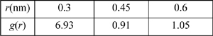
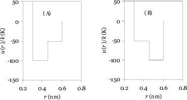
8.38. Suppose two molecules had similar potential functions, but they were mirror images of one another as shown in the figure below. Which one (A or B) would have the larger internal energy departure? You may assume that the radial distribution function is the same for both potential models.
a. Reason qualitatively but refer to appropriate equations to explain your answer.
b. Compute the values of (U – Uig)/RT at a packing fraction of 0.4 and a temperature of 50 K. Assume values of the radial distribution function as follows: