
Chapter 9. Phase Equilibrium in a Pure Fluid
One of the principal objects of theoretical research is to find the point of view from which it can be expressed with greatest simplicity.
J.W. Gibbs (1881)
The problem of phase equilibrium is distinctly different from “(In – Out) = Accumulation.” The fundamental balances were useful in describing many common operations like throttling, pumping, and compressing, and fundamentally, they provide the basis for understanding all processes. But the balances make a relatively simple contribution in solving problems of phase equilibrium—so much so that they are largely ignored, while simple questions like “How many phases are present?” take the primary role.
The general problem of phase equilibrium has a broad significance that begins to distinguish chemical thermodynamics from more generic thermodynamics. If we only care about steam, then it makes sense to concentrate on the various things we can do with steam and to use the steam tables for any properties we need. But, if our interest is in a virtually infinite number of chemicals and mixtures, then we need some unifying principles. Since our interest is chemical thermodynamics, we must deal extensively with property estimations. The determination of phase equilibrium is one of the most important and difficult estimations to make. The ability to understand, model, and predict phase equilibria is particularly important for designing separation processes. Typically, these operations comprise the most significant capital costs of plant facilities, and require knowledgeable engineers to design, maintain, and troubleshoot them.
In most separation processes, the controlled variables are the temperature and pressure. Thus, when we approach the modeling of phase behavior, we should seek thermodynamic properties that are natural functions of these two properties. In our earlier discussions of convenience properties, the Gibbs energy was shown to be such a function:
As a defined mathematical property, the Gibbs energy remains abstract, in the same way that enthalpy and entropy are difficult to conceptualize. However, our need for a natural function of P and T requires the use of this property.
![]() Phase equilibrium at fixed T and P is most easily understood using G, which is a natural function of P, T.
Phase equilibrium at fixed T and P is most easily understood using G, which is a natural function of P, T.
Chapter Objectives: You Should Be Able to...
1. Use the Clapeyron and Clausius-Clapeyron equations to calculate thermodynamic properties from limited data.
2. Explain the origin of the shortcut vapor pressure equation and its limitations.
3. Use the Antoine equation to calculate saturation temperature or saturation pressure.
4. Describe in words the relationship between the Gibbs departure and the fugacity.
5. Given the pressure and temperature, estimate the value of fugacity (in appropriate units) using an ideal gas model, virial correlation, or cubic equation of state.
6. Calculate the fugacity coefficient of a vapor or liquid given an expression for a cubic equation of state and the parameter values Z, A, B, and decide which root among multiple roots is most stable.
7. Estimate the fugacity of a liquid or solid if given the vapor pressure.
8. Interpret equation of state results at saturation and apply the lever rule to properties like enthalpy, internal energy, and entropy for a two-phase mixture.
9. Solve throttling, compressor, and turbine expander problems using a cubic equation of state for thermodynamic properties rather than a chart or table.
9.1. Criteria for Phase Equilibrium
As an introduction to the constraint of phase equilibrium, let us consider an example. A piston/cylinder contains both propane liquid and vapor at –12°C. The piston is forced down a specified distance. Heat transfer is provided to maintain isothermal conditions. Both phases still remain. How much does the pressure increase?
This is a trick question. As long as two phases are present for a single component and the temperature remains constant, then the system pressure remains fixed at the vapor pressure, so the answer is zero increase. The molar volumes of vapor and liquid phases also stay constant since they are state properties. However, as the total volume changes, the quantity of liquid increases, and the quantity of vapor decreases. We are working with a closed system where n = nL + nV. For the whole system: V = nL VsatL + nVVsatV = n·VsatL + q·n·(VsatV – VsatL) and since VsatL and VsatV are fixed and VsatL < VsatV, a decrease in V causes a decrease in q1.
Since the temperature and pressure from beginning to end are constant as long as two phases exist, applying Eqn. 9.1 shows that the change in Gibbs energy of each phase of the system from beginning to end must be zero, dGL = dGV = 0.
For the whole system:
But by the mass balance, dnL = –dnV which reduces Eqn. 9.2 to 0 = GL – GV or
This is a very significant result. In other words, GL = GV is a constraint for phase equilibrium. None of our other thermodynamic properties, U, H, S, and A is equivalent in both phases. If we specify phase equilibrium must exist and one additional constraint (e.g., T), then all of our other state properties of each phase are fixed and can be determined by the equation of state and heat capacities.
Only needing to specify one variable at saturation to compute all state properties should not come as a surprise, based on our experience with the steam tables. The constraint of GL = GV is simply a mathematical way of saying “saturated.” As an exercise, select from the steam tables an arbitrary saturation condition and calculate G = H – TS for each phase. The advantage of the mathematical expression is that it yields a specific equality applicable to many chemicals. The powerful insight of GL = GV leads us to the answers of many more difficult and significant questions concerning phase equilibrium.
9.2. The Clausius-Clapeyron Equation
We can apply these concepts of equilibrium to obtain a remarkably simple equation for the vapor-pressure dependence on temperature at low pressures. As a “point of view of greatest simplicity,” the Clausius-Clapeyron equation is an extremely important example. Suppose we would like to find the slope of the vapor pressure curve, dPsat/dT. Since we are talking about vapor pressure, we are constrained by the requirement that the Gibbs energies of the two phases remain equal as the temperature is changed. If the Gibbs energy in the vapor phase changes, the Gibbs energy in the liquid phase must change by the same amount. Thus,
dGL = dGV
Rewriting the fundamental property relation ⇒ dG = VV dPsat – SV dT = VL dPsat – SL dT and rearranging,
Entropy is a difficult property to measure. Let us use a fundamental property to substitute for entropy. By definition of G: GV = HV – TSV = HL – TSL = GL
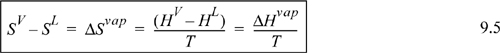
Substituting Eqn. 9.5 in for SV – SL in Eqn. 9.4, we have the Clapeyron equation which is valid for pure fluids along the saturation line:

Note: This general form of Clapeyron equation can be applied to any kind of phase equilibrium including solid-vapor and solid-liquid equilibria by substituting the alternative sublimation or fusion properties into Eqn. 9.6; we derived the current equation based on vapor-liquid equilibria.
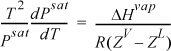
Several simplifications can be made in the application to vapor pressure (i.e., vapor-liquid equilibium). To write the equation in terms of ZV and ZL, we multiply both sides by T2 and divide both sides by Psat:
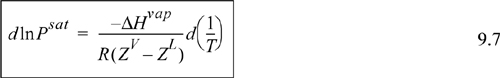
We then use calculus to change the way we write the Clapeyron equation:
Combining the results, we have an alternative form of the Clapeyron equation:
For a gas far from the critical point at “low” reduced temperatures, ZV – ZL ≈ ZV. In addition, for vapor pressures near 1 bar, where ideal gas behavior is approximated, ZV ≈ 1, resulting in the Clausius-Clapeyron equation:

Example 9.1. Clausius-Clapeyron equation near or below the boiling point
Derive an expression based on the Clausius-Clapeyron equation to predict vapor-pressure dependence on temperature.
Solution
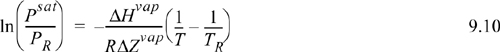
If we assume that ΔHvap is fairly constant in some range near the boiling point, integration of each side of the Clausius-Clapeyron equation can be performed from the boiling point to another state on the saturation curve, which yields
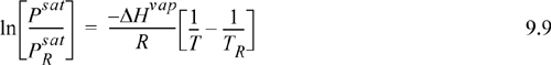
where ![]() is 0.1013 MPa and TR is the normal boiling temperature. This result may be used in a couple of different ways: (1) We may look up ΔHvap so that we can calculate Psat at a new temperature T; or (2) we may use two vapor pressure points to calculate ΔHvap and subsequently apply method (1) to determine other Psat values.
is 0.1013 MPa and TR is the normal boiling temperature. This result may be used in a couple of different ways: (1) We may look up ΔHvap so that we can calculate Psat at a new temperature T; or (2) we may use two vapor pressure points to calculate ΔHvap and subsequently apply method (1) to determine other Psat values.
One vapor pressure point is commonly available through the acentric factor, which is the reduced vapor pressure at a reduced temperature of 0.7. (Frequently the boiling point is near this temperature.) That means, we can apply the definition of the acentric factor to obtain a value of the vapor pressure relative to the critical point.
9.3. Shortcut Estimation of Saturation Properties
We found that the Clausius-Clapeyron equation leads to a simple, two-constant equation for the vapor pressure at low temperatures. What about higher temperatures? Certainly, the assumption of ideal gases used to derive the Clausius-Clapeyron equation is not valid as the vapor pressure becomes large at high temperature; therefore, we need to return to the Clapeyron equation. If ΔHvap/ΔZvap was constant over a wide range of temperature, then we could recover this simple form. Obviously, ΔZvap is not constant; as we approach the critical point, the vapor and liquid volumes get closer together until they eventually become equal and ΔZvap → 0. However, the enthalpies of the vapor and liquid approach one another at the critical point, so it is possible that ΔHvap/ΔZvap may be approximately constant. To analyze this hypothesis, let us plot the experimental data in the form of Eqn. 9.7 assuming that ΔHvap/ΔZvap is constant. A constant slope would confirm a constant value of ΔHvap/ΔZvap. A plot is shown for two fluids in Fig. 9.1.
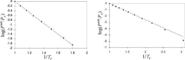
Figure 9.1. Plot to evaluate Clausius-Clapeyron for calculation of vapor pressures at high pressures, argon (left) and ethane (right).
The conclusion is that setting ΔH/ΔZ equal to a constant is a reasonable approximation, especially over the range of 0.5 < Tr < 1.0. The plot for ethane shows another nearly linear region for 1/Tr > 2 (temperatures below the normal boiling temperature), with a different slope and intercept. The approach of the previous section should be applied at Tr < 0.5. Integrating the Clapeyron equation for vapor pressure, we obtain,
Example 9.2. Vapor pressure interpolation
What is the value of the pressure in a piston/cylinder at –12°C (261.2 K) with vapor and liquid propane present? Use only the boiling temperature (available from a handbook), critical properties, and acentric factor to determine the answer.
We will use the boiling point and the vapor pressure given by the acentric factor to determine (–ΔHvap)/(RΔZvap) for Eqn. 9.10, and then use the boiling temperature with (–ΔHvap)/(RΔZvap) to determine the desired vapor pressure. First, let us use the acentric factor to determine the vapor pressure value at Tr = 0.7. For propane, Tc = 369.8 K, Pc = 4.249 MPa, and ω = 0.152. Solving for the vapor pressure in terms of MPa by rearranging the definition of the acentric factor, ![]() MPa.a The temperature corresponding to this pressure is T = Tr·Tc = 0.7·369.8 = 258.9 K. The CRC handbook lists the normal boiling temperature of propane as –42°C = 231.2 K. Using these two vapor pressures in Eqn. 9.10:
MPa.a The temperature corresponding to this pressure is T = Tr·Tc = 0.7·369.8 = 258.9 K. The CRC handbook lists the normal boiling temperature of propane as –42°C = 231.2 K. Using these two vapor pressures in Eqn. 9.10:
ln(0.2994/0.1013) = –ΔHvap/(RΔZvap)(1/258.9 – 1/231.2) ⇒ –ΔHvap/(RΔZ) = –2342 K
Therefore, using the boiling point and the value of –ΔHvap/(RΔZvap),
Psat(261.2 K) = 0.1013 MPa · exp[–2342(1/261.2 – 1/231.2)] = 0.324 MPa
The calculation is in excellent agreement with the experimental value of 0.324 MPa.
a. Could we use the Clausius-Clapeyron equation at this condition? Since the Clausius-Clapeyron equation requires the ideal gas law, the Psat value must be low enough for the ideal gas law to be followed. The deviations at this state can be quickly checked with the virial equation, Pr = 0.07, Tr = 0.7, B0 = –0.664, B1 = –0.630, Z = 0.924; therefore, the Clausius-Clapeyron equation should probably not be used. Although you would get the same answer for vapor pressure over this narrow range, your inaccurate estimate of ΔHvap might mislead you in a later calculation.
Since the linear relationship of Eqn. 9.10 applies over a broad range of temperatures, we can derive an approximate general estimate of the saturation pressure based on the critical point as the reference and acentric factor as a second point on the vapor pressure curve.
Setting PR = Pc and TR = Tc,
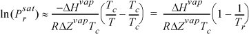
Common logarithms are conventional for shortcut estimation, possibly because they are more convenient to visualize orders of magnitude.
Relating this equation to the acentric factor defined by Eqn. 7.2,
which results in a shortcut vapor pressure equation,
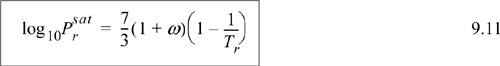
Note: The shortcut vapor pressure equation must be regarded as an approximation for rapid estimates. The approximation is generally good above P = 0.5 bar; the percent error can become significant at lower pressures (and temperatures). Keep in mind that its estimates are based on the critical pressure which is generally 40–50 bar and acentric factor (at Tr = 0.7).
Example 9.3. Application of the shortcut vapor pressure equation
Use the shortcut vapor pressure equation to calculate the vapor pressure of propane at –12°C, and compare the calculation with the results from Example 9.2.
Solution
For propane at –12oC, Tr = 261.2/369.8 = 0.7063,
This is in excellent agreement with the result of Example 9.2, with considerably less effort.
Example 9.4. General application of the Clapeyron equation
Liquid butane is pumped to a vaporizer as a saturated liquid under a pressure of 1.88 MPa. The butane leaves the exchanger as a wet vapor of 90 percent quality and at essentially the same pressure as it entered. From the following information, estimate the heat load on the vaporizer per gram of butane entering.
For butane, Tc = 425.2 K; Pc = 3.797 MPa; and ω = 0.193. Use the shortcut method to estimate the temperature of the vaporizer, and the Peng-Robinson equation to determine the enthalpy of vaporization.
Solution
To find the T at which the process occurs:a
First, we use the Peng-Robinson equation to find departure functions for each phase, and subsequently determine the heat of vaporization at 383.2 K and 1.88 MPa:
Therefore, ΔHvap = (–0.9949 + 5.256)8.314·0.90117·425.2 = 13,575 J/mol
Since the butane enters as saturated liquid and exits at 90% quality, an energy balance gives Q = 0.9·13,575 = 12,217 J/mol ·1mol/58g = 210.6 J/g
Alternatively, we could have used the shortcut equation another way by comparing the Clapeyron and shortcut equations:
Clapeyron: ln(Psat) = –ΔHvap/RT(ZV – ZL) + ΔHvap/RTc(ZV – ZL) + lnPc
Shortcut: ![]()
Comparing, we find: ![]()
Therefore, using the Peng-Robinson equation at 383.3 K and 1.88 MPa to determine compressibility factor values,
ΔHvap = 2725R (ZV – ZL) = 2725(8.314)(0.6744 – 0.07854) = 13,500 J/mol
which would give a result in good agreement with the first approach.
a. In principle, since we are asked to use the Peng-Robinson equation for the rest of the problem, we could have used it to determine the saturation temperature also, but we were asked to use the shortcut method. The use of equations of state to calculate vapor pressure is discussed in Section 8.10.
The Antoine Equation
The simple form of the shortcut vapor-pressure equation is extremely appealing, but there are times when we desire greater precision than such a simple equation can provide. One obvious alternative would be to use the same form over a shorter range of temperatures. By fitting the local slope and intercept, an excellent fit could be obtained. To extend the range of applicability slightly, one modification is to introduce an additional adjustable parameter in the denominator of the equation. The resultant equation is referred to as the Antoine equation:
![]() Antoine equation. Use with care outside the stated parameter temperature limits, and watch use of log, ln, and units carefully.
Antoine equation. Use with care outside the stated parameter temperature limits, and watch use of log, ln, and units carefully.
where T is conventionally in Celsius.2 Values of coefficients for the Antoine equation are widely available, notably in the compilations of vapor-liquid equilibrium data by Gmehling and coworkers.3 The Antoine equation provides accurate correlation of vapor pressures over a narrow range of temperatures, but a strong caution must be issued about applying the Antoine equation outside the stated temperature limits; it does not extrapolate well. If you use the Antoine equation, you should be sure to report the temperature limits as well as the values of coefficients with every application. Antoine coefficients for some compounds are summarized in Appendix E and within the Excel workbook Antoine.xlsx.
9.4. Changes in Gibbs Energy with Pressure
We have seen that the Gibbs energy is the key property that must be used to characterize phase equilibria. In the previous section, we have used Gibbs energy in the derivation of useful relations for vapor pressure. For our discussions here, we have been able to relate the two phases of a pure fluid to one another, and the actual calculation of values of the Gibbs energy were not needed. However, extension to general phase equilibria in the next chapters will require a capability to calculate departures of Gibbs energies of individual phases, sometimes using different techniques of calculation for each phase.
By observing the mathematical behavior of Gibbs energy for fluids derived from the above equations, some sense may be developed for how pressure affects Gibbs energy, and the property becomes somewhat more tangible. Beginning from our fundamental relation, dG = –SdT + VdP, the effect of pressure is most easily seen at constant temperature.
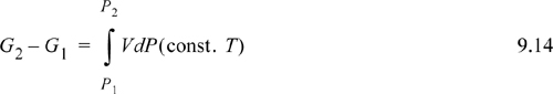
Eqn. 9.13 is the basic equation used as a starting point for derivations used in phase equilibrium. In actual applications the appearance of the equation may differ, but it is useful to recall that most derivations originate with the variation of Eqn. 9.13. To evaluate the change in Gibbs energy, we simply need the P-V-T properties of the fluid. These P-V-T properties may be in the form of tabulated data from measurements, or predictions from a generalized correlation or an equation of state. For a change in pressure, Eqn. 9.13 may be integrated:
Methods for calculating Gibbs energies and related properties differ for gases, liquids, and solids. Each type of phase will be covered in a separate section to make the distinctions of the calculation methods clearer. Before proceeding to those analyses, however, we consider a problem which arises in the treatment of Gibbs energy at low pressure. This problem motivates the introduction of the term “fugacity” which takes the place of the Gibbs energy in the presentation in the following sections.
Gibbs Energy in the Low-Pressure Limit
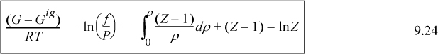
The calculation of ΔG is illustrated in Fig. 9.2, where the shaded area represents the integral. The slope of a G versus P plot at constant temperature is equal to the molar volume. For a real fluid, the ideal-gas approximation is valid only at low pressures. The volume is given by V = ZRT/P; thus,
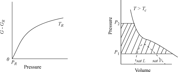
Figure 9.2. Schematic of dependence of G on pressure for a real fluid at TR, and an isothermal change on a P-V diagram for a change from P1 to P2.
which permits use of generalized correlations or volume-explicit equations of state to represent Z at T and P.4 Of course, we may also use Eqn. 9.13 directly, using an equation of state to calculate V. Both techniques are shown later, but first the qualitative aspects of the calculations are illustrated.
For an ideal gas, we may substitute Z = 1 into Eqn. 9.15 to obtain
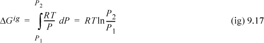
Both dG and dGig become infinite as pressure approaches zero. This means that both Eqns. 9.15 and 9.16 are difficult to use directly at low pressure. However, as a real fluid state approaches zero pressure, Z will approach the ideal gas limit and dG approaches dGig. Thus, the difference dG – dGig will remain finite, and goes to zero as P goes to zero. Thus,
dG – dGig = d(G – Gig)
which is simply the change in departure function. Therefore, we combine Eqns. 9.15 and 9.16 and write:
This relates the departure function to the P-V-T properties in a way that we have seen before. If you look back to Eqn. 8.26, that equation looks different because we are integrating over volume rather than pressure, but they are really related. We use this departure to define a new state property, fugacity, to describe phase behavior. We reserve further discussion of pressure effects in gases for the following sections, where fugacity and Gibbs energy can be considered simultaneously. The generalized treatment by departure functions is also discussed there.
9.5. Fugacity and Fugacity Coefficient
In principle, all pure-component, phase-equilibrium problems could be solved using Gibbs energy. Historically, however, an alternative property has been applied in chemical engineering calculations, the fugacity. The fugacity has one advantage over the Gibbs energy in that its application to mixtures is a straightforward extension of its application to pure fluids. It also has some empirical appeal because the fugacity of an ideal gas equals the pressure and the fugacity of a liquid equals the vapor pressure under common conditions, as we will show in Section 9.8. The vapor pressure was the original property used for characterization of phase equilibrium by experimentalists.
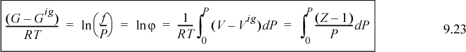
The forms of Eqns. 9.16 and 9.15 are similar, and the simplicity of Eqn. 9.16 is appealing. G.N. Lewis defined fugacity by
and comparing to Eqn. 9.16, we see that
Integrating from low pressure, at constant temperature, we have for the left-hand side,
because (G – Gig) approaches zero at low pressure. Integrating the right-hand side of Eqn. 9.20, we have
To complete the definition of fugacity, we define the low-pressure limit,
and we define the ratio f/P to be the fugacity coefficient, ϕ.

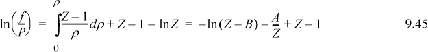
The fugacity coefficient is simply another way of characterizing the Gibbs departure function at a fixed T,P. For an ideal gas, the fugacity will equal the pressure, and the fugacity coefficient will be unity. For representations of the P-V-T data in the form Z = f(T,P) (like the virial equation of state), the fugacity coefficient is evaluated from an equation of the form:
or the equivalent form for P-V-T data in the form Z = f(T,V), which is essentially Eqn. 8.26,
which is the form used for cubic equations of state.
A graphical interpretation of the fugacity coefficient can be seen in Fig. 9.3. The integral of Eqn. 9.23 is represented by the negative value of the shaded region between the real gas isotherm and the ideal gas isotherm. The fugacity coefficient is a measure of non-ideality. Under most common conditions, the fugacity coefficient is less than one. At very high pressures, the fugacity coefficient can become greater than one.
Figure 9.3. Illustration of RT ln ϕ as a departure function.
Note: In practice, we do not evaluate the fugacity of a substance directly. Instead, we evaluate the fugacity coefficient, and then calculate the fugacity by
9.6. Fugacity Criteria for Phase Equilibria
We began the chapter by showing that Gibbs energy was equivalent in phases at equilibrium. Here we show that equilibrium may also be described by equivalence of fugacities. Since
we may subtract Gig from both sides and divide by RT, giving
Substituting Eqn. 9.22,
which becomes
Therefore, calculation of fugacity and equating in each phase becomes the preferred method of calculating phase equilibria. In the next few sections, we discuss the methods for calculation of fugacity of gases, liquids, and solids.
9.7. Calculation of Fugacity (Gases)
The principle of calculation of the fugacity coefficient is the same by all methods—Eqn. 9.23 or 9.24 is evaluated. The methods look considerably different, usually because the P-V-T properties are summarized differently. All methods use the formula below and differ only in the manner the fugacity coefficient is evaluated.
Equations of State
Equations of state are the dominant method used in process simulators because the EOS can be solved rapidly by computer. We consider two equations of state, the virial equation and the Peng-Robinson equation. We also consider the generalized compressibility factor charts as calculated with the Lee-Kesler equation.
Ideal Gas
The Virial Equation
The virial equation may be used to represent the compressibility factor in the low-to-moderate pressure region where Z is linear with pressure at constant temperature. Eqn. 7.10 should be used to evaluate the appropriateness of the virial coefficient method. Substituting Z = 1 + BP/RT, or Z – 1 = BP/RT into Eqn. 9.23,

Thus,
Writing the virial coefficient in reduced temperature and pressure,

where B0 and B1 are the virial coefficient correlations given in Eqns. 7.8 and 7.9 on page 259.
The Peng-Robinson Equation
Cubic equations of state are particularly useful in the petroleum and hydrocarbon-processing industries because they may be used to represent both vapor and liquid phases. Chapter 7 discussed how equations of state may be used to represent the volumetric properties of gases. The integral of Eqn. 9.23 is difficult to use for pressure-explicit equations of state; therefore, it is solved in the format of Eqn. 9.24. The integral is evaluated analytically by methods of Chapter 8. In fact, the result of Example 8.6 on page 317 is ln ϕ according to the Peng-Robinson equation.

To apply, the technique is analogous to the calculation of departure functions. At a given P, T, the cubic equation is solved for Z, and the result is used to calculate ϕ and then fugacity is calculated, f = ϕP. This method has been programmed into Preos.xlsx and Preos.m.
Below the critical temperature, equations of state may also be used to predict vapor pressure, saturated vapor volume, and saturated liquid volume, as well as liquid volumetric properties. While Eqn. 9.33 can be used to calculate fugacity coefficients for liquids, the details of the calculation will be discussed in the next section. Note again that Eqn. 9.24 is closely related to Eqn. 8.26 as used in Example 8.6 on page 317.
Generalized Charts
Properties represented by generalized charts may help to visualize the magnitudes of the fugacity coefficient in various regions of temperature and pressure. To use the generalized chart, we write
The Gibbs energy departure chart can be generated from the Lee-Kesler equation by specifying a particular value for the acentric factor. The charts are for the correlation ln ϕ = ln ϕ0 + ωln ϕ1. The entropy departure can also be estimated by combining Fig. 9.4 with Fig. 8.7:
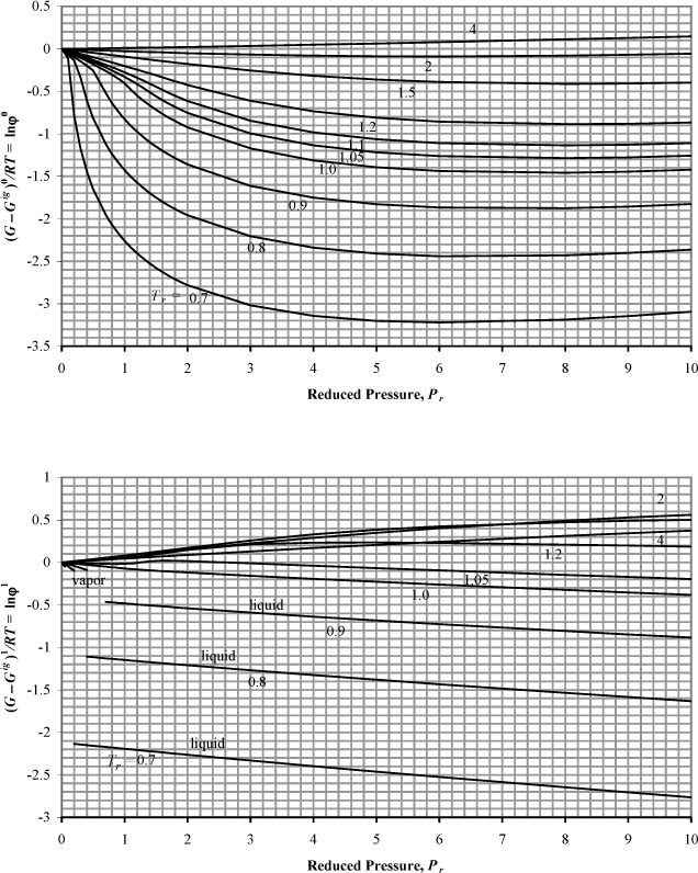
Figure 9.4. Generalized charts for estimating the Gibbs departure function using the Lee-Kesler equation of state. (G – Gig)0/RT uses ω = 0.0, and (G – Gig)1/RT is the correction factor for a hypothetical compound with ω = 1.0.
Fig. 9.4 can be useful for hand calculation, if you do not have a computer. A sample calculation for propane at 463.15 and 2.5 MPa gives
compared to the value of –0.112 from the Peng-Robinson equation.
9.8. Calculation of Fugacity (Liquids)
To introduce the calculation of fugacity for liquids, consider Fig. 9.5. The shape of an isotherm below the critical temperature differs significantly from an ideal-gas isotherm. Such an isotherm is illustrated which begins in the vapor region at low pressure, intersects the phase boundary where vapor and liquid coexist, and then extends to higher pressure in the liquid region. Point A represents a vapor state, point B represents saturated vapor, point C represents saturated liquid, and point D represents a liquid.
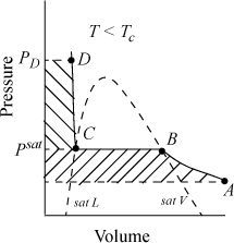
Figure 9.5. Schematic for calculation of Gibbs energy and fugacity changes at constant temperature for a pure liquid.
We showed in Section 9.6 on page 346 that
Note that we have designated the fugacity at points C and B equal to fsat. This notation signifies a saturation condition, and as such, it does not require a distinction between liquid or vapor. Therefore, we may refer to point B or C as saturated vapor or liquid interchangeably when we discuss fugacity. The calculation of the fugacity at point B (saturated vapor) is also adequate for calculation of the fugacity at point C, the fugacity of saturated liquid. Calculation of the saturation fugacity may be carried out by any of the methods for calculation of vapor fugacities from the above section. Methods differ slightly on how the fugacity is calculated between points C and D. There are two primary methods for calculating this fugacity change. They are the Poynting method and the equation of state method.
Poynting Method
The Poynting method applies Eqn. 9.19 between saturation (points B, C) and point D. The integral is
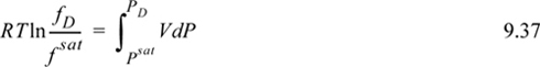
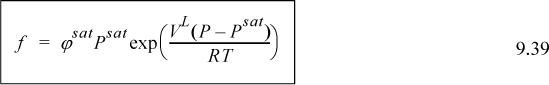
Since liquids are fairly incompressible for Tr < 0.9, the volume is approximately constant, and may be removed from the integral, with the resultant Poynting correction becoming

The fugacity is then calculated by
Saturated liquid volume can be estimated within a slight percent error using the Rackett equation
The Poynting correction, Eqn. 9.38, is essentially unity for many compounds near room T and P; thus, it is frequently ignored.
Equation of State Method
Calculation of liquid fugacity by the equation of state method uses Eqn. 9.24 just as for vapor. To apply the Peng-Robinson equation of state, we can use Eqn. 9.33. The only significant consideration is that the liquid compressibility factor must be used. To understand the mathematics of the calculation, consider the isotherm shown in Fig. 9.6(a). When Tr < 1, the equation of state predicts an isotherm with “humps” in the vapor/liquid region. Surprisingly, these swings can encompass a range of negative values of the pressure near C′ (although not shown in our example). The exact values of these negative pressures are not generally taken too seriously, however, because they occur in a region of the P-V diagram that is unimportant for routine calculations. Since the Gibbs energy from an equation of state is given by an integral of the volume with respect to pressure, the quantity of interest is represented by an integral of the humps. The downward and upward humps cancel one another in generating that integral. This observation gives rise to the equal area rule for computing saturation conditions to be discussed in Section 9.10 where we show that the shaded area above line ![]() is equal to the shaded area below, and that the pressure where the line is located represents the saturation condition (vapor pressure). With regard to fugacity calculations, it is sufficient simply to note that these humps are in fact integrable, and easily computed by the same formula derived for the vapor fugacity by an equation of state.
is equal to the shaded area below, and that the pressure where the line is located represents the saturation condition (vapor pressure). With regard to fugacity calculations, it is sufficient simply to note that these humps are in fact integrable, and easily computed by the same formula derived for the vapor fugacity by an equation of state.
Fig. 9.6(b) shows that the molar Gibbs energy is indeed continuous as the fluid transforms from the vapor to the liquid. The Gibbs energy first increases according to Eqn. 9.14 based on the vapor volume. Note that the volume and pressure changes are both positive, so the Gibbs energy relative to the reference value is monotonically increasing. During the transition from vapor to liquid, the “humps” lead to the triangular region associated with the name of van der Waals loop. Then the liquid behavior takes over and Eqn. 9.14 comes back into play, this time using the liquid volume. Note that the isothermal pressure derivative of the Gibbs energy is not continuous. Can you develop a simple expression for this derivative in terms of P, V, T, CP, CV, and their derivatives? Based on your answer to the preceding question, would you expect the change in the derivative to be a big change or a small change?

Figure 9.6. Schematic illustration of the prediction of an isotherm by a cubic equation of state. Compare with Fig. 9.5 on page 350. The figure on the right shows the calculation of Gibbs energy relative to a reference state. The fugacity will have the same qualitative shape.
Example 9.5. Vapor and liquid fugacities using the virial equation
Determine the fugacity (MPa) for acetylene at (a) 250 K and 10 bar, and (b) 250 K and 20 bar. Use the virial equation and the shortcut vapor pressure equation.
Solution
From the back flap of the text for acetylene: Tc = 308.3 K, Pc = 6.139, ω = 0.187, Zc = 0.271. For each part of the problem, the fluid state of aggregation is determined before the method of solution is specified. At 250 K, using the shortcut vapor pressure equation, Eqn 9.11, the vapor pressure is Psat = 1.387 MPa.
We will calculate the virial coefficient at 250 K using Eqns. 7.7–7.9:
Tr = 250/308.3 = 0.810, Bo = –0.5071, B1 = –0.2758, B = –233.3 cm3/mol.
a. P = 1 MPa < Psat so the acetylene is vapor (between points A and B in Fig. 9.5). Using Eqn 7.10 to evaluate the appropriateness of the virial equation at 1 MPa, Pr = 1/6.139 = 0.163, and 0.686 + 0.439Pr = 0.76 and Tr = 0.810, so the correlation should be accurate.
Using Eqn. 9.31,
(f = ϕ P = 0.894 (1) = 0.894 MPa
b. P = 2 MPa > Psat, so the acetylene is liquid (point D of Fig. 9.5). For a liquid phase, the only way to incorporate the virial equation is to use the Poynting method, Eqn. 9.39. Using Eqn. 7.10 to evaluate the appropriateness of the virial equation at the vapor pressure, Prsat = 1.387/6.139 = 0.2259, and 0.686 + 0.439Prsat = 0.785, and Tr = 0.810, so the correlation should be accurate.
At the vapor pressure,
fsat = ϕsat Psat = 0.8558(1.387) = 1.187 MPa
Using the Poynting method to correct for pressure beyond the vapor pressure will require the liquid volume, estimated with the Rackett equation, Eqn. 9.40, using Vc = ZcRTc/Pc = 0.271(8.314)(308.3)/6.139 = 113.2 cm3/mol.
The Poynting correction is given by Eqn. 9.38,
Thus, f = 1.187(1.015) = 1.20 MPa. The fugacity is close to the value of vapor pressure for liquid acetylene, even though the pressure is 2 MPa.
9.9. Calculation of Fugacity (Solids)
Fugacities of solids are calculated using the Poynting method, with the exception that the volume in the Poynting correction is the volume of the solid phase.

Any of the methods for vapors may be used for calculation of ϕsat. Psat is obtained from thermodynamic tables. Equations of state are generally not applicable for calculation of solid phases because they are used only to represent liquid and vapor phases. However, they may be used to calculate the fugacity of a vapor phase in equilibrium with a solid, given by ϕsatPsat. As for liquids, the Poynting correction may be frequently set to unity with negligible error.

9.10. Saturation Conditions from an Equation of State
The only thermodynamic specification that is required for determining the saturation temperature or pressure is that the Gibbs energies (or fugacities) of the vapor and liquid be equal. This involves finding the pressure or temperature where the vapor and liquid fugacities are equal. The interesting part of the problem comes in computing the saturation condition by iterating on the temperature or pressure.
Example 9.6. Vapor pressure from the Peng-Robinson equation
Use the Peng-Robinson equation to calculate the normal boiling point of methane.
Solution
Vapor pressure calculations are available in Preos.xlsx and PreosPropsmenu.m. Let us discuss Preos.xlsx first. The spreadsheet is more illustrative in showing the steps to the calculation. Computing the saturation temperature or pressure in Excel is rapid using the Solver tool in Excel.
On the spreadsheet shown in Fig. 9.7, cell H12 is included with the fugacity ratio of the two phases; the cell can be used to locate a saturation condition. Initialize Excel by entering the desired P in cell B8, in this case 0.1 MPa. Then, adjust the temperature to provide a guess in the two-phase (three-root) region. Then, instruct Solver to set the cell for the fugacity ratio (H12) to a value of one by adjusting temperature (B7), subject to the constraint that the temperature (B7) is less than the critical temperature.

Figure 9.7. Example of Preos.xlsx used to calculate vapor pressure.
In MATLAB, the initial guess is entered in the upper left. The “Run Type” is set as a saturation calculation. The “Root to use” and “Value to match” are not used for a saturation calculation. The drop-down box “For Matching...” is set to adjust the temperature. The results are shown in Fig. 9.8.

Figure 9.8. Example of PreosPropsMenu.m used to calculate vapor pressure.
For methane the solution is found to be 111.4 K which is very close to the experimental value used in Example 8.9 on page 320. Saturation pressures can also be found by adjusting pressure at fixed temperature.
Fugacity and P-V isotherms for CO2 as calculated by the Peng-Robinson equation are shown in Fig. 9.9 and Fig. 7.5 on page 264. Fig. 9.9 shows more clearly how the shape of the isotherm is related to the fugacity calculation. Note that the fugacity of the liquid root at pressures between B and B′ of Fig. 9.6 is lower than the fugacity of the vapor root in the same range, and thus is more stable because the Gibbs energy is lower. Analogous comparisons of vapor and liquid roots at pressures between C and C′ show that vapor is more stable. In Chapter 7, we empirically instructed readers to use the lower fugacity. Now, in light of Fig. 9.9, readers can understand the reasons for the use of fugacity.

Figure 9.9. Predictions of the Peng-Robinson equation of state for CO2: (a) prediction of the P-V isotherm and fugacity at 280 K; (b) plot of data from part (a) as fugacity versus pressure, showing the crossover of fugacity at the vapor pressure. Several isotherms for CO2 are shown in Fig. 7.5 on page 264.
The term “fugacity” was defined by G. N. Lewis based on the Latin for “fleetness,” which is often interpreted as “the tendency to flee or escape,” or simply “escaping tendency.” It is sometimes hard to understand the reasons for this term when calculating the property for a single root. However, when multiple roots exist as shown in Fig. 9.9, you may be able to understand how the system tries to “escape: from the higher fugacity values to the lower values. This perspective is especially helpful in mixtures, indicating the direction of driving forces to lower fugacities.
Just as the vapor pressure estimated by the shortcut vapor pressure equation is less than 100% accurate, the vapor pressure estimated by an equation of state is less than 100% accurate. For example, the Peng-Robinson equation tends to yield about 5% average error over the range 0.4 < Tr < 1.0. This represents a significant improvement over the shortcut equation. The van der Waals equation, on the other hand, yields much larger errors in vapor pressure. One problem is that the van der Waals equation offers no means of incorporating the acentric factor to fine-tune the characterization of vapor pressure. But the problems with the van der Waals equation go much deeper, as illustrated in the example below.
Example 9.7. Acentric factor for the van der Waals equation
To clarify the problem with the van der Waals equation in regard to phase-equilibrium calculations, it is enlightening to compute the reduced vapor pressure at a reduced temperature of 0.7. Then we can apply the definition of the acentric factor to characterize the vapor pressure behavior of the van der Waals equation. If the acentric factor computed by the van der Waals equation deviates significantly from the acentric factor of typical fluids of interest, then we can quickly assess the magnitude of the error by applying the shortcut vapor-pressure equation. Perform this calculation and compare the resulting acentric factor to those on the inside covers of the book.
Solution
The computations for the van der Waals equation are very similar to those for the Peng-Robinson equation. We simply need to derive the appropriate expressions for a0, a1, and a2, that go into the analytical solution of the cubic equation: Z3+ a2 Z2 + a1 Z + a0 = 0.
Adapting the procedure for the Peng-Robinson equation given in Section 7.6 on page 263, we can make Eqn. 7.13 dimensionless:
where the dimensionless parameters are given by Eqns. 7.21–7.24; A = (27/64) Pr/Tr2; B = 0.125 Pr/Tr.
After writing the cubic in Z, the coefficients can be identified: a0 = –AB; a1 = A; and a2 = –(1 + B). For the calculation of vapor pressure, the fugacity coefficient for the van der Waals equation is quickly derived as the following:
Substituting these relations in place of their equivalents in Preos.xlsx, the problem is ready to be solved. Since we are not interested in any specific compound, we can set Tc = 1 and Pc = 1, Tr = 0.7. Setting an initial guess of Pr = 0.1, Solver gives the result that Pr = 0.20046.
Modification of PreosPropsMenu.m is accomplished by editing the routine PreosProps.m. Search for the text “global constants.” Change the statements to match the a and b for the van der Waals equation. Search for “PRsolveZ” Two cases will be calls and you may wish to change the function name to “vdwsolveZ.” The third case of “PRsolveZ” will be the function that solves the cubic. Change the function name. Edit the formulas used for the cubic coefficients. Finally, specify a fluid and find the vapor pressure at the temperature corresponding to Tr = 0.7.
The definition of the acentric factor gives
ω = –log(Pr) – 1 = –log(0.20046) – 1 = –0.302
Comparing this value to the acentric factors listed in the table on the back flap, the only compound that even comes close is hydrogen, for which we rarely calculate fugacities at Tr < 1. This is the most significant shortcoming of the van der Waals equation. This shortcoming becomes most apparent when attempting to correlate phase-equilibria data for mixtures. Then it becomes very clear that accurate correlation of the mixture phase equilibria is impossible without accurate characterization of the pure component phase equilibria, and thus the van der Waals equation by itself is not useful for quantitative calculations. Correcting the repulsive contribution of the van der Waals equation using the Carnahan-Starling or ESD form gives significant improvement in the acentric factor. Another approach is to correct the attractive contribution in a way that cancels the error of the repulsive contribution. Cancellation is the approach that historically prevailed in the Redlich-Kwong, Soave, and Peng-Robinson equations.
The Equal Area Rule
As noted above, the swings in the P-V curve give rise to a cancellation in the area under the curve that becomes the free energy/fugacity. A brief discussion is helpful to develop an understanding of how the saturation pressure and liquid and vapor volumes are determined from such an isotherm.
To make this analysis quantitative, it is helpful to recall the formulas for the Gibbs departure functions, noting that the Gibbs departure is equal for the vapor and liquid phases (Eqn. 9.26).


In the final equation, the second term in the right-hand side braces represents the area under the isotherm, and the first term on the right-hand side represents the rectangular area described by drawing a horizontal line at the saturation pressure from the liquid volume to the vapor volume in Fig. 9.6(a). Since this area is subtracted from the total inside the braces, the shaded area above a vapor pressure is equal to the shaded area below the vapor pressure for each isotherm. This method of computing the saturation condition is very sensitive to the shape of the P-V curve in the vicinity of the critical point and can be quite useful in estimating saturation properties at near-critical conditions.
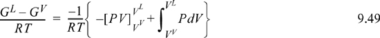
Although Eqn. 9.49 illustrates the concept of the equal area rule most clearly, it is not in the form that is most useful for practical application. Noting that GL = GV at equilibrium and rearranging Eqn. 9.47 gives
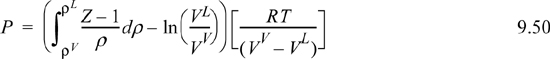
You should recognize the first term on the right-hand side as (AL – Aig)T,V – (AV – Aig)T,V. You probably have an expression for (A – Aig)T,V already derived. Solving for P is iterative in nature because we must first guess a value for P to solve for VV and VL. Five or six iterations normally suffice to converge to reasonable precision.5 The method is guaranteed to converge as long as a maximum and minimum exist in the P-V isotherm. Therefore, initiation begins with finding the extrema, a form of “stability check” (see below) in the sense that the absence of extrema indicates a single phase. The search for extrema is facilitated by noting that the vapor maximum must appear at ρ < ρc while the liquid minimum must appear at ρ < ρc. If Pmin > 0, then initialize to P0 = (Pmin+Pmax)/2. Otherwise, initialize by finding VV and VL at P = 10–12. The procedure is applied in Example 9.8 below.
Example 9.8. Vapor pressure using equal area rule
Convergence can be tricky near the critical point or at very low temperatures when using the equality of fugacity, as in Example 9.6. The equal area rule can be helpful in those situations. As an example, try calling the solver for CO2 at 30°C. Even though the initial guess from the shortcut equation is very good, the solver diverges. Alternatively, apply the equal area rule to solve as described above. Conditions in this range may be “critical” to designing CO2 refrigeration systems, so reliable convergence is important.
Solution
The first step is to construct an isotherm and find the spinodal densities and pressures. Fig. 9.10 shows that Pmin = 7.1917, Pmax = 7.2291, Vmax = 117.98, and Vmin = 94.509. Following the procedure above, P0 = 7.2104. Solving for the vapor and liquid roots at P0 in the usual way gives Vvap = 129.842, and Vliq = 88.160. Similarly, (AL – Aig)T,V = –1.0652 and (AV – Aig)T,V. = –0.7973, referring to the formula given in Example 8.6 on page 317:
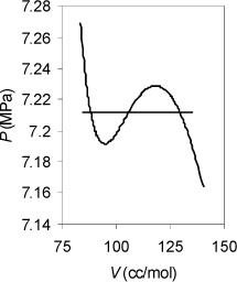
Figure 9.10. Illustration of use of the equal area rule for a small van der Waals loop.
This leads to the next estimate of Psat as,
Psat = [–1.0652 + 0.7973 – ln(88.160/129.842)][8.314(303.15)/(129.842 – 88.160)] = 7.2129
Solving for the vapor and liquid roots and repeating twice more gives: Psat = 7.21288, shown below. Note the narrow range of pressures.
9.11. Stable Roots and Saturation Conditions
When multiple real roots exist, the fugacity is used to determine which root is stable as explained in Section 9.10. However, often we are seeking a value of a state property and we are unable to find a stable root with the target value. This section explains how we handle that situation. We use entropy for the discussion, but calculations with other state properties would be similar.
Fig. 9.11 shows the behavior of the entropy values for ethane at 0.1 MPa as calculated by the Peng-Robinson equation of state using a real gas reference state of T = 298.15K and P = 0.1 MPa. The figure was generated from the spreadsheet Preos.xlsx by adding the formula for entropy departure for the center root and then changing the temperature at a fixed pressure of 0.1 MPa. The corresponding values of S were recorded and plotted.
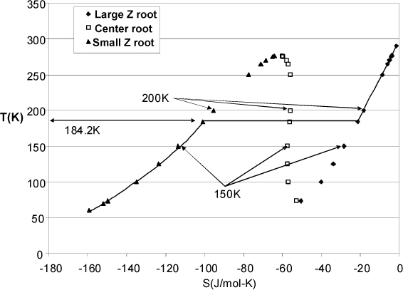
Figure 9.11. Entropy values for ethane calculated from the Peng-Robinson equation along an isobar at 0.1 MPa. The largest Z root is shown as diamonds, the smallest Z root is shown as triangles, and the center root is shown as open squares. The stable behavior is indicated by the solid line.
Suppose a process problem requires a state with S = –18.185 J/mol-K. At 200 K, the largest Z root has this value. The corresponding values of the fugacities from largest to smallest Z are 0.0976 MPa, 0.652 MPa, and 0.206 MPa, indicating that the largest root is most stable, so the largest root will give the remainder of the state variables.
Suppose a process problem requires a state with S = –28.35 J/mol-K. At 150 K, the largest Z root has this value. The corresponding values of the fugacities from largest to smallest Z are 0.0951 MPa, 0.313 MPa, and 0.0099 MPa, indicating that the smallest root is most stable. Even though the largest Z root has the correct value of S, the root is not the most stable root, and must be discarded.
Further exploration of roots would show that the desired value of S cannot be obtained by the middle or smallest roots, or any most stable root. Usually if this behavior is suspected, it is quickest to determine the saturation conditions for the given pressure and compare the saturation values to the specified value. (Think about how you handled saturated steam calculations from a turbine using the steam tables and used the saturation values as a guide.) The saturation conditions at 0.1 MPa can be found by adjusting the T until the fugacities become equal for the large Z and small Z roots, which is found to occur at 184.2 K. At this condition, the corresponding values of the fugacities from largest to smallest Z are 0.0971 MPa, 0.524 MPa, and 0.0971 MPa, indicating that largest and smallest Z roots are in phase equilibrium, and the center root is discarded as before. The corresponding values for saturated entropy are S = –21.3021 J/mol-K for the vapor phase and –100.955 J/mol-K for the liquid phase. For any condition at 0.1 MPa, any value of S between these two values will fall in the two-phase region. Therefore, the desired state of S = –28.35 J/mol-K is two-phase, with a quality calculated using the saturation values,
S = SsatL + q (SsatV – SsatL)
–28.35 J/mol-K = –100.955 + q(–21.3021 + 100.955). Solving, q = 0.912
The cautions highlighted in the example also apply when searching for specific values of other state properties by adjusting P and/or T. For example, it is also common to search for a state with specified values of {H,P} by adjusting T. The user must make sure that the root selected is a stable root, or if the system is two-phase, then a quality calculation must be performed.6
9.12. Temperature Effects on G and f
The effect of temperature at fixed pressure is
The Gibbs energy change with temperature is then dependent on entropy. Gibbs energy will decrease with increasing temperature. Since the entropy of a vapor is higher than the entropy of a liquid, the Gibbs energy will change more rapidly with temperature for vapor. Since the Gibbs energy is proportional to the log of fugacity, the fugacity dependence will follow the same trends. Similar statements are valid comparing liquids and solids.7
9.13. Summary
We began this chapter by introducing the need for Gibbs energy to calculate phase equilibria in pure fluids because it is a natural function of temperature and pressure. We also introduced fugacity, which is a convenient property to use instead of Gibbs energy because it resembles the vapor pressure more closely. We also showed that the fugacity coefficient is directly related to the deviation of a fluid from ideal gas behavior, much like a departure function (Eqns. 9.23 and 9.24). This principle of characterization of non-ideality extends into the next chapter where we consider non-idealities of mixtures. In fact, much of the pedagogy presented in this chapter finds its significance in the following chapters, where the phase equilibria of mixtures become much more complex.
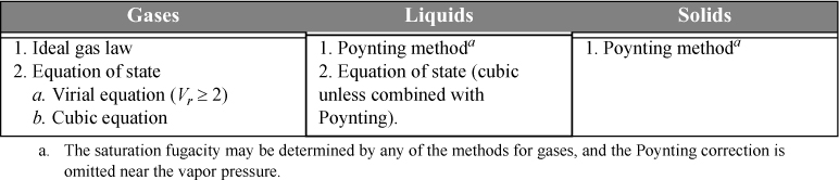
Methods for calculating fugacities were introduced using charts, equations of state, and derivative manipulations. (In the homework problems, we offer illustration of how tables may also be used.) Liquids and solids were considered in addition to gases, and the Poynting correction was introduced for calculating the effect of pressure on condensed phases. These pure component methods are summarized in Table 9.1, and they are applied often in the analysis of mixtures. Skills in their application must be kept ready throughout the following chapters.
Table 9.1. Techniques for Calculation Pure Component Fugacities
A critical concept in this chapter is that when multiple EOS roots exist from a process calculation, the stable root has a lower Gibbs energy or lower fugacity. We also provided methods to find saturation conditions for pure fluids.
Important Equations
Eqns. 9.3 and 9.27 basically state that equilibrium occurs when fugacity in each phase is equal. This is a general principle that can be applied to components in mixtures and forms the basis for phase equilibrium computations in mixtures. Eqn. 9.11 is a special form of Eqn. 9.6 that is particularly convenient for estimating the vapor pressure over wide ranges of temperature. It may not be as precise as the Antoine equation over a narrow temperature range, but it is less likely to lead to a drastic error when extrapolation is necessary. Nevertheless, Eqn. 9.11 is not a panacea. When you are faced with phase equilibrium problems other than vapor pressure, like solid-liquid (e.g., melting ice) or solid-vapor (e.g., dry ice), you must start with Eqn. 9.6 and re-derive the final equations subject to relevant assumptions for the problem of interest.
Fugacity is commonly calculated by Eqns. 9.28(Gases), 9.29(Ideal gases), 9.41(Liquids), and 9.43(Solids), and is dependent on the calculation of the fugacity coefficient. Fugacity is particularly helpful in identifying the stable root.
9.14. Practice Problems
P9.1. Carbon dioxide (CP = 38 J/mol-K) at 1.5 MPa and 25°C is expanded to 0.1 MPa through a throttle valve. Determine the temperature of the expanded gas. Work the problem as follows:
a. Assuming the ideal gas law (ANS. 298 K)
b. Using the Peng-Robinson equation (ANS. 278 K, sat L + V)
c. Using a CO2 chart, noting that the triple point of CO2 is at –56.6°C and 5.2 bar, and has a heat of fusion, ΔHfus, of 43.2 cal/g. (ANS. 194 K, sat S + V)
P9.2. Consider a stream of pure carbon monoxide at 300 bar and 150 K. We would like to liquefy as great a fraction as possible at 1 bar. One suggestion has been to expand this high-pressure fluid across a Joule-Thompson valve and take what liquid is formed. What would be the fraction liquefied for this method of operation? What entropy is generated per mole processed? Use the Peng-Robinson equation. Provide numerical answers. Be sure to specify your reference state. (Assume CP = 29 J/mol-K for a quick calculation.) (ANS. 32% liquefied)
P9.3. An alternative suggestion for the liquefaction of CO discussed above is to use a 90% efficient adiabatic turbine in place of the Joule-Thomson valve. What would be the fraction liquefied in that case? (ANS. 60%)
P9.4. At the head of a methane gas well in western Pennsylvania, the pressure is 250 bar, and the temperature is roughly 300 K. This gas stream is similar to the high-pressure stream exiting the precooler in the Linde process. A perfect heat exchanger (approach temperature of zero) is available for contacting the returning low-pressure vapor stream with the incoming high-pressure stream (similar to streams 3–8 of Example 8.9 on page 320). Compute the fraction liquefied using a throttle if the returning low-pressure vapor stream is 30 bar. (ANS. 30%)
9.15. Homework Problems
9.1. The heat of fusion for the ice-water phase transition is 335 kJ/kg at 0°C and 1 bar. The density of water is 1g/cm3 at these conditions and that of ice is 0.915 g/cm3. Develop an expression for the change of the melting temperature of ice as a function of pressure. Quantitatively explain why ice skates slide along the surface of ice for a 100 kg hockey player wearing 10 cm x 01 cm blades. Can it get too cold to ice skate? Would it be possible to ice skate on other materials such as solid CO2?
9.2. Thermodynamics tables and charts may be used when both H and S are tabulated. Since G = H – TS, at constant temperature, ΔG = RT ln(f2/f1) = ΔH – TΔS. If state 1 is at low pressure where the gas is ideal, then f1 = P1, RT ln(f2/P1) = ΔH – TΔS, where the subscripts indicate states. Use this method to determine the fugacity of steam at 400°C and 15 MPa. What value does the fugacity coefficient have at this pressure?
9.3. This problem reinforces the concepts of phase equilibria for pure substances.
a. Use steam table data to calculate the Gibbs energy of 1 kg saturated steam at 150°C, relative to steam at 150°C and 50 kPa (the reference state). Perform the calculation by plotting the volume data and graphically integrating. Express your answer in kJ. (Note: Each square on your graph paper will represent [pressure·volume] corresponding to the area, and can be converted to energy units.)
b. Repeat the calculations using the tabulated enthalpies and entropies. Compare your answer to part (a).
c. The saturated vapor from part (a) is compressed at constant T and 1/2 kg condenses. What is the total Gibbs energy of the vapor liquid mixture relative to the reference state of part (a)? What is the total Gibbs energy relative to the same reference state when the mixture is completely condensed to form saturated liquid?
d. What is the Gibbs energy of liquid water at 600 kPa and 150°C relative to the reference state from part (a)? You may assume that the liquid is incompressible.
e. Calculate the fugacities of water at the states given in parts (a) and (d). You may assume that f = P at 50 kPa.
9.4. Derive the formula for fugacity according to the van der Waals equation.
9.5. Use the result of problem 9.4 to calculate the fugacity of ethane at 320 K and at a molar volume of 150 cm3/mole. Also calculate the pressure in bar.
9.6. Calculate the fugacity of ethane at 320 K and 70 bar using:
a. Generalized charts
b. The Peng-Robinson equation
9.7. CO2 is compressed at 35°C to a molar volume of 200 cm3/gmole. Use the Peng-Robinson equation to obtain the fugacity in MPa.
9.8. Use the generalized charts to obtain the fugacity of CO2 at 125°C and 220 bar.
9.9. Calculate the fugacity of pure n-octane vapor as given by the virial equation at 580 K and 0.8 MPa.
9.10. Estimate the fugacity of pure n-pentane (C5H12) at 97°C and 7 bar by utilizing the virial equation.
9.11. Develop tables for H, S, and Z for N2 over the range Pr = [0.5, 1.5] and Tr = [Trsat, 300 K] according to the Peng-Robinson equation. Use the saturated liquid at 1 bar as your reference condition for H = 0 and S = 0.
9.12. Develop a P-H chart for saturated liquid and vapor butane in the range T = [260, 340] using the Peng-Robinson equation. Show constant S lines emanating from saturated vapor at 260 K, 300 K, and 340 K. For an ordinary vapor compression cycle, what would be the temperature and state leaving an adiabatic, reversible compressor if the inlet was saturated vapor at 260 K? (Hint: This is a tricky question.)
9.13. Compare the Antoine and shortcut vapor-pressure equations for temperatures from 298 K to 500 K. (Note in your solution where the equations are extrapolated.) For the comparison, use a plot of log10Psat versus 1/T except provide a separate plot of Psat versus T for vapor pressures less than 0.1 MPa.
a. n-Hexane
b. Acetone
c. Methanol
d. 2-propanol
e. Water
9.14. For the compound(s) specified by your instructor in problem 9.13, use the virial equation to predict the virial coefficient for saturated vapor and the fugacity of saturated liquid. Compare the values of fugacity to the vapor pressure.
9.15. Compare the Peng-Robinson vapor pressures to the experimental vapor pressures (represented by the Antoine constants) for the species listed in problem 9.13.
9.16. Carbon dioxide can be separated from other gases by preferential absorption into an amine solution. The carbon dioxide can be recovered by heating at atmospheric pressure. Suppose pure CO2 vapor is available from such a process at 80°C and 1 bar. Suppose the CO2 is liquefied and marketed in 43-L laboratory gas cylinders that are filled with 90% (by mass) liquid at 295 K. Explore the options for liquefaction, storage, and marketing via the following questions. Use the Peng-Robinson for calculating fluid properties. Submit a copy of the H-U-S table for each state used in the solution.
a. Select and document the reference state used throughout your solution.
b. What is the pressure and quantity (kg) of CO2 in each cylinder?
c. A cylinder marketed as specified needs to withstand warm temperatures in storage/transport conditions. What is the minimum pressure that a full gas cylinder must withstand if it reaches 373 K?
d. Consider the liquefaction process via compression of the CO2 vapor from 80°C, 1 bar to 6.5 MPa in a single adiabatic compressor (ηC = 0.8). The compressor is followed by cooling in a heat exchanger to 295 K and 6.5 MPa. Determine the process temperatures and pressures, the work and heat transfer requirement for each step, and the overall heat and work.
e. Consider the liquefaction via compression of the CO2 vapor from 80°C, 1 bar to 6.5 MPa in a two-stage compressor with interstage cooling. Each stage (ηC = 0.8) operates adiabatically. The interstage pressure is 2.5 MPa, and the interstage cooler returns the CO2 temperature to 295 K. The two-stage compressor is followed by cooling in a heat exchanger to 295 K and 6.5 MPa. Determine all process temperatures and pressures, the work and heat transfer requirement for each step, and the overall heat and work.
f. Calculate the minimum work required for the state change from 80°C, 1 bar to 295 K, 6.5 MPa with heat transfer to the surroundings at 295 K. What is the heat transfer required with the surroundings?
9.17. A three-cycle cascade refrigeration unit is to use methane (cycle 1), ethylene (cycle 2), and ammonia (cycle 3). The evaporators are to operate at: cycle 1, 115.6 K; cycle 2, 180 K; cycle 3, 250 K. The outlets of the compressors are to be: cycle 1, 4 MPa; cycle 2, 2.6 MPa; cycle 3, 1.4 MPa. Use the Peng-Robinson equation to estimate fluid properties. Use stream numbers from Fig. 5.11 on page 212. The compressors have efficiencies of 80%.
a. Determine the flow rate for cycle 2 and cycle 3 relative to the flow rate in cycle 1.
b. Determine the work required in each compressor per kg of fluid in the cycle.
c. Determine the condenser duty in cycle 3 per kg of flow in cycle 1.
d. Suggest two ways that the cycle could be improved.
9.18. Consider the equation of state
where ηp = b/V.
a. Determine the relationships between a, b, c and Tc, Pc, Zc.
b. What practical restrictions are there on the values of Zc that can be modeled with this equation?
c. Derive an expression for the fugacity.
d. Modify Preos.xlsx or Preos.m for this equation of state. Determine the value of c (+/- 0.5) that best represents the vapor pressure of the specified compound below. Use the shortcut vapor pressure equation to estimate the experimental vapor pressure for the purposes of this problem for the option(s) specifed by your instructor.
i. CO2
ii. Ethane
iii. Ethylene
iv. Propane
v. n-Hexane