
Chapter 13. Local Composition Activity Models
I have constructed three thousand different theories in connection with the electric light... Yet, in only two cases did my experiments prove the truth of my theory.
Thomas A. Edison
It is evident from Chapter 12 that describing solution nonideality with van der Waals’ mixing rules is imprecise. With a single parameter like k12 or A12, we can match the magnitude of the excess energy, but not the skewness. The Margules two-parameter and van Laar models address this problem in an ad hoc fashion, but there is no physical basis for extending these to multiple components. A rational basis for extending the analysis of mixtures should seek a legitimate explanation for the source of varied skewness. One such explanation is that molecules do not distribute themselves randomly. Instead, they may tend to form clusters. You might witness this kind of distribution at a dinner party, where the children are in one area, the men are discussing sports, and the ladies are discussing anything but sports. There is sufficient mixing among the clusters that you cannot consider it a phase separation. Some children and ladies like sports. Some men do not. Nevertheless, the distribution is not entirely random. In other words, the local composition around a child at a dinner party, for example, may differ from the bulk composition. We examine this prospect graphically in Example 13.2. Local composition models recognize this possibility and account for the local composition enhancement in terms of two parameters, just enough to characterize both the magnitude and the skewness of the excess energy. Careful analysis of the molecular scale energies in terms of the local compositions facilitates straightforward extension to multicomponent mixtures.
Chapter Objectives: You Should Be Able to...
1. Characterize adjustable parameters in local composition activity models using experimental data.
2. Comment critically on the merits and limitations of the following activity models: Wilson, UNIQUAC, UNIFAC, and NRTL, including the ability to identify the most appropriate model for a given mixture.
A Preliminary Glimpse of UNIFAC — A Predictive Method
This chapter is densely packed with theoretical details. In the interest of “telling you what we are going to tell you,” it is useful to see how the final equations are applied before being concerned with their derivations. One popular activity coefficient model is the predictive model of UNIFAC. It is the closest thing to a universally applicable predictive model that we currently have, so it makes sense to get right to the point and introduce the rudiments of implementing this model at an early stage. It is a rather complicated model and deriving it must await several other derivations. Nevertheless, the availability of a computer program for applying the method makes it possible to apply it as a “black box” at this stage, and the utility of the model should inspire us to learn more about it. Detailed calculations are illustrated in the UNIFAC spreadsheet in the file Actcoeff.xlsx introduced in Chapter 11, and in the MATLAB file Ex13_01.m.
Example 13.1. VLE prediction using UNIFAC activity coefficients
The 2-propanol (also known as isopropyl alcohol or IPA) + water (W) system is known to form an azeotrope at atmospheric pressure and 80.37°C (xW = 0.3146).a Use UNIFAC to estimate the conditions of the azeotrope at 760 mmHg. Is UNIFAC accurate for this mixture?
Solution
The Antoine coefficients for IPA and water are given in Appendix E. To begin, the VLE can be computed at the true experimental conditions to see if it looks like there is an azeotrope nearby. This system is presented in Figs. 10.8 and 10.9, so we know what the answer looks like. We will use the principles developed in Section 11.7 to determine if an azeotrope exists. Note that the azeotrope condition is at a maximum or minimum on the diagrams.
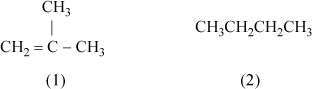
The pressure is given as 760 mmHg. We develop a detailed description of the UNIFAC model later, but you need to know a little bit about it just to run the program. The UNIFAC model is based on structural and energetic information for the functional groups that comprise the molecules in the mixture. The UNIFAC model estimates the activity coefficients using the groups by calculating size, shape, and energy parameters based on the number and types of groups in the molecules.b The structures of the molecules for this problem and the UNIFAC groups are:
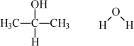

The UNIFAC model can be operated from either the Excel spreadsheet or the MATLAB routine. To operate the spreadsheet program, simply type the temperature of interest (80.37) and the number of functional groups of each type in the appropriate column for each component. In MATLAB, the groups are entered into the cell matrix compArray. Group names available in MATLAB can be determined by using load 'unifacAij.mat'.
Enter the mole fractions (e.g., [xW = 0.3146, xIPA = 0.6854]). The activity coefficients are ⇒ γw = 2.1108; γIPA = 1.0885. According to modified Raoult’s law, ![]() . By entering the proper Antoine coefficients, the pressure is computed using this formula, and we can keep guessing temperatures (which changes γs and Psats) until the pressure equals 760 mmHg (or we can apply the Excel solver tool or MATLAB fzero ⇒ T = 80.47°C):
. By entering the proper Antoine coefficients, the pressure is computed using this formula, and we can keep guessing temperatures (which changes γs and Psats) until the pressure equals 760 mmHg (or we can apply the Excel solver tool or MATLAB fzero ⇒ T = 80.47°C):
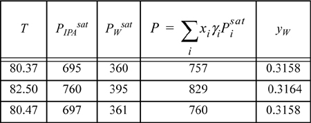
The vapor phase mole fractions are calculated using ![]() and an analogous expression for the second component (or by using y2 = 1 – y1). Since the vapor and liquid compositions are not equal (xw = 0.3146 ≠ 0.3158 = yw), we did not find the azeotrope. We must try several values of x to find the azeotrope composition.
and an analogous expression for the second component (or by using y2 = 1 – y1). Since the vapor and liquid compositions are not equal (xw = 0.3146 ≠ 0.3158 = yw), we did not find the azeotrope. We must try several values of x to find the azeotrope composition.
Try xw = 0.3177 ⇒ γW = 2.1035; γIPA = 1.0904:

Since xw = 0.3177 = yw, this is the composition of the azeotrope estimated by UNIFAC. UNIFAC seems to be fairly accurate for this mixture at the azeotrope. Also note that T versus x is fairly flat near an azeotrope; this is why it was unnecessary to modify the guess for bubble temperature at the new composition. This is generally true, and important in the distillation of azeotropic systems.
a. Perry, R.H., Chilton, C.H. 1973. Chemical Engineers’ Handbook, 5 ed, New York NY: McGraw-Hill, Chapter 13.
b. The functional groups for a given molecule are often determined automatically by process design software. Several examples of group assignments are given in Table 13.2 on page 512.
13.1. Local Composition Theory
Now that we see the capabilities of the predictions, we have motivation to understand the model. One of the major assumptions of van der Waals mixing was that the mixture interactions were independent of each other such that quadratic mixing rules would provide reasonable approximations as shown in Eqn. 12.3 on page 467. But in some cases, like radically different strengths of attraction, the mixture interaction can be strongly coupled to the mixture composition. That is, for instance, the cross parameter could be a function of composition: a12 = a12(x). One way of treating this prospect is to recognize the possibility that the local compositions in the mixture might deviate strongly from the bulk compositions. As an example, consider a lattice consisting primarily of type A atoms but with two B atoms right beside each other. Suppose all these atoms were the same size and that the coordination number was 10. Then the local compositions around a B atom are xAB = 9/10 and xBB = 1/10 (notation of subscripts is AB ⇒ “A around B”). Specific interactions such as hydrogen bonding and polarity might lead to such effects, and thus, the basis of the hypothesis is that energetic differences lead to the nonrandomness that causes the quadratic mixing rules to break down. To develop the theory, we first introduce nomenclature to identify the local compositions summarized in Table 13.1.
Table 13.1. Nomenclature for Local Composition Variables

We assume that the local compositions are given by some weighting factor, Ωij, relative to the overall compositions.
Therefore, if Ω12 = Ω21 = 1, the solution is random. Before introducing the functions that describe the weighting factors, let us discuss how the factors may be used.
Local Compositions around “1” Molecules
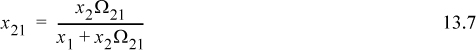
Let us begin by considering compositions around “1” molecules. We would like to write the local mole fractions x21 and x11 in terms of the overall mole fractions, x1 and x2. Using the local mole balance,
Rearranging Eqn. 13.1,
Substituting Eqn. 13.4 into Eqn. 13.3,
Rearranging,
Substituting Eqn. 13.6 into Eqn. 13.4,
Local Compositions around “2” Molecules
Similar derivations for molecules of type “2” results in

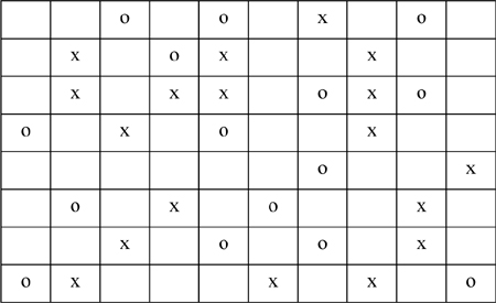
Example 13.2. Local compositions in a two-dimensional lattice
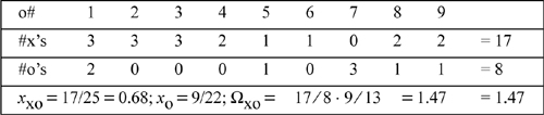
The following lattice contains x’s, o’s, and void spaces. The coordination number of each cell is 8. Estimate the local composition (xxo) and the parameter Ωxo based on rows and columns away from the edges.

Solution
There are 9 o’s and 13 x’s that are located away from the edges. The number of x’s and o’s around each o are as follows:
Note: Fluids do not really behave as though their atoms were located on lattice sites, but there are many theories based on the supposition that lattices represent reasonable approximations. In this text, we have elected to omit detailed treatment of lattice theory on the basis that it is too approximate to provide an appreciation for the complete problem and too complicated to justify treating it as a simple theory. This is a judgment call and interested students may wish to learn more about lattice theory. Sandler presents a brief introduction to the theory which may be acceptable for readers at this level.a
a. Sandler, S.I. 1989. Chemical Entineering Thermodynamic, 2nd ed. Hoboken NJ: Wiley.
Local Composition and Gibbs Energy of Mixing
We need to relate the local compositions to the excess Gibbs energy. The perspective of representing all fluids by the square-well potential lends itself naturally to the local composition concept. Then the intermolecular energy is given simply by the local composition times the well-depth for that interaction. We simply ignore all but the nearest neighbors because they are outside the square-well. In equation form, the energy equation for mixtures can be reformulated in terms of local compositions. The local mole fraction can be related to the bulk mole fraction by defining a quantity Ωij as follows:
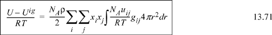
The next step in the derivation requires scaling up from the molecular-scale local composition to the macroscopic energy in the mixture. The rigorous procedure for taking this step requires integration of the molecular distributions times the molecular interaction energies, analogous to the procedure for pure fluids as applied in Section 7.11. This rigorous development is presented below in Section 13.7. On the other hand, it is possible to simply present the result of that derivation for the time being. This permits a more rapid exploration of the practical implications of local composition theory. The form of the equation is not so difficult to understand from an intuitive perspective, however. The energy departure is simply a multiplication of the local composition (xij) by the local interaction energy (εij). The departure properties are calculated based on a general model known as the two-fluid theory.1 According to the two-fluid theory, any intensive departure function in a binary is given by
Where the local composition environment of the type 1 molecules determines (M–Mig)(1), and the local composition environment of the type 2 molecules determines (M–Mig)(2). Note that (M–Mig)(i) is composition-dependent and is equal to the pure component value only when the local composition is pure i.
Using the concept of a square-well model and thus counting only nearest neighbors, noting that ε12 = ε21, and recalling that the local mole fractions must sum to unity, we have for a binary mixture
where Nc,j is the coordination number (total number of atoms in the neighborhood of the jth species), and where we can identify
When x1 approaches unity, x2 goes to zero, and from Eqn. 13.1 x21 goes to zero, and x11 goes to one. The limits applied to Eqn. 13.11 result in (U – Uig)pure1 = (NA/2)Nc,1ε11. Similarly, when x2 approaches unity, (U – Uig)pure2 = (NA/2)Nc,2ε22. For an ideal solution,
The excess energy is obtained by subtracting Eqn. 13.13 from Eqn. 13.11,
Collecting terms with the same energy variables, and using the local mole balance from Table 13.1 on page 502, (x11–1)ε11 = –x21ε11, and (x22–1)ε22 = –x12ε22, resulting in
Substituting Eqn. 13.7 and Eqn. 13.8,

At this point, the traditional local composition theories deviate from regular solution theory in a way that really has nothing to do with local compositions. Instead, the next step focuses on one of the subtleties of classical thermodynamics. Example 6.7 shows that the derivative of Helmholtz energy is related to internal energy. Therefore, we can integrate energy to find the change in Helmholtz energy,

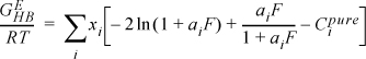
where ![]() is the infinite temperature limit at the given liquid density, independent of temperature but possibly dependent on composition or density. We need to insert Eqn. 13.16 into Eqn. 13.17 and integrate. We need to have some algebraic expression for the dependence of Ωij on temperature, which is what distinguishes the local composition theories from each other.
is the infinite temperature limit at the given liquid density, independent of temperature but possibly dependent on composition or density. We need to insert Eqn. 13.16 into Eqn. 13.17 and integrate. We need to have some algebraic expression for the dependence of Ωij on temperature, which is what distinguishes the local composition theories from each other.
13.2. Wilson’s Equation
Wilson2 made a bold assumption regarding the temperature dependence of Ωij. Wilson’s original parameter used in the literature is Λji, but it is related to Ωij in a very direct way. Wilson assumes3

(note: Λii = Λjj = 1, and Aij ≠ Aji even though εij = εji), and integration with respect to T becomes very simple. Assuming Nc,j = 2 for all j at all ρ,

A convenient simplifying assumption before proceeding further is that GE ~ AE. This corresponds to neglecting the excess volume of mixing relative to the other contributions and is quite acceptable for liquids. The customary way of interpreting GE/RT is to separate it into an energetic part known as the residual contribution, (GE/RT)RES, that vanishes at infinite temperature or when ε12 – ε22 = 0 and ε21 – ε11 = 0, and a size/shape part known as the combinatorial contribution, (GE/RT)COMB, that represents the infinite temperature limit at the liquid density. For Wilson’s equation, the first two terms vanish at high T, so
For the combinatorial contribution, Wilson used Flory’s equation,
It should be noted that the assumption of the temperature dependence of Eqn. 13.18 has been made for convenience, but there is some justification for it, as we show in Section 13.7. Wilson’s equation becomes

Algebraic rearrangement of Wilson’s equation results in the form that is usually cited,
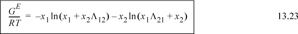
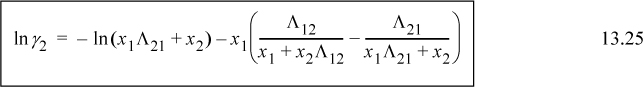
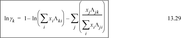
For a binary system, the activity coefficients from the Wilson equation are:

Noting that Λ11 = Λ22 = 1, and looking back at Eqn. 13.6, we can also see that for the first equation ![]() . We can rearrange this expression to obtain the slightly more compact relation:
. We can rearrange this expression to obtain the slightly more compact relation:

Similar rearrangement of the second expression gives:
![]() Parameters for the Wilson equation, Aji. Note that the literature values often include energy units. Use the correct R!
Parameters for the Wilson equation, Aji. Note that the literature values often include energy units. Use the correct R!
One limitation of Wilson’s equation is that it is unable to model liquid-liquid equilibria, but it is reasonably accurate for modeling the liquid phase when correlating the vapor liquid equilibria.
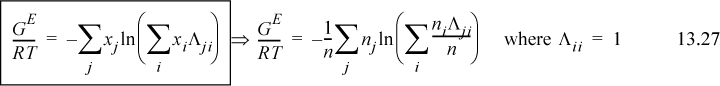
Extending Eqn. 13.23 to a multicomponent solution,
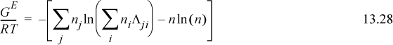
To determine activity coefficients, the excess Gibbs energy is differentiated. Differentiating the last term,
and letting “sum” stand for the summation of Eqn. 13.28, and combining,
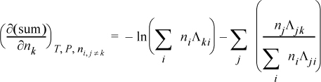
combining,
Example 13.3. Application of Wilson’s equation to VLE
For the binary system n-pentanol(1) + n-hexane(2), the Wilson equation constants are A12 = 1718 cal/mol, A21 = 166.6 cal/mol. Assuming the vapor phase to be an ideal gas, determine the composition of the vapor in equilibrium with a liquid containing 20 mole% n-pentanol at 30°C. Also calculate the equilibrium pressure. ![]() ;
; ![]() .
.
Solution
From CRC,
ρ1 = 0.8144 g/ml (1mole/88g) ⇒ V1 = 108 cm3/mole
ρ2 = 0.6603 g/ml (1mole/86g) ⇒ V2 = 130 cm3/mole
Note: ρ1 and ρ2 are functions of T but ρ1/ρ2 ≈ const. ⇒ V2/V1 = 1.205 assumed at all T.
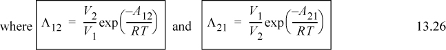
Utilizing Eqn. 13.26,
Λ12 = 1.205 exp(– 1718/1.987/303) = 0.070; Λ21 = 1/1.205 exp(– 166.6/1.987/303) = 0.629
In γ1 = 1.0408 ⇒ γ1 = 2.822; In γ2 = 0.1584 ⇒ γ2 = 1.172
y1 = x1γ1Psat/P = 0.2·2.822·3.23/177.2 = 0.0103
13.3. NRTL
The NRTL model4 (short for Non-Random Two Liquid) equates UE from Eqn. 13.16 directly to GE, ignoring the proper thermodynamic integration. At the same time, it introduces a third binary parameter that generates an extremely flexible functional form for fitting activity coefficients.

For a binary mixture, the activity equations become

For a binary mixture, the activity equations become


When αij = 0, the binary model simplifies to the one-parameter Margules model,
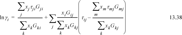
The NRTL model is not very appealing from a theoretical perspective, but its flexibility has led to a broad range of applications including combinations with electrolyte models. As a practical matter, a value of αij = 0.3 is taken as a default and the equation works much like the Wilson equation, except that it is able to model LLE. The parameter αij is adjusted for additional flexibility when necessary, such as when modeling LLE where the value is commonly increased. The multicomponent form of NRTL is
13.4. UNIQUAC
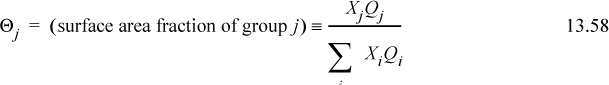
UNIQUAC5 (short for UNIversal QUAsi Chemical model) builds on the work of Wilson by making three primary refinements. First, the temperature dependence of Ωij is modified to depend on surface areas rather than volumes, based on the hypothesis that the interaction energies that determine local compositions are dependent on the relative surface areas of the molecules. If the parameter qi is proportional to the surface area of molecule i,

where z = 10. The intermediate parameter τij = exp(– aij/T) is used for compact notation where τii = τjj = 1, aii = ajj = 0.6 In addition, when the energy equation 13.16 is written with Nc,j = zqj = 10qj for all j at all ρ, the different sizes and shapes of the molecules are implicitly taken into account. Qualitatively, the number of molecules that can contact a central molecule increases as the size of the molecule increases. Using surface fractions attempts to recognize the branching and overlap that can occur between segments in a polyatomic molecule. The inner core of these segments is not accessible, only the surface is accessible for energetic interactions. Therefore, the model of the energy is proposed to be proportional to surface area. Unfortunately, it is not straightforward to construct a more rigorous argument in favor of surface fractions from the energy equation itself. Inserting Eqns. 13.31 and 13.16 into Eqn. 13.17, the excess Helmholtz for a binary solution becomes
where θi is the surface area fraction, and θi = xiqi/(x1q1 + x2q2) for a binary. Analogous to Wilson’s equation, GE is calculated as AE, a good approximation. The first two terms represent (GE/RT)RES,
that can be compared with Eqn. 13.20 and the final term ![]() represents (GE/RT)COMB. The (GE/RT)COMB term is attributed to the entropy of mixing hard chains, and an approximate expression for this contribution is applied by Maurer and Prausnitz.7 This representation of the entropy of mixing traces its roots back to the work of Staverman8 and Guggenheim9 and was discussed more recently by Lichtenthaler et al.10 It is very similar to the Flory term, but it corrects for the fact that large molecules are not always large balls, but sometimes long “strings.” By noting that the ratio of surface area to volume for a sphere is different from that for a string, Guggenheim’s form (the form actually applied in UNIFAC and UNIQUAC) provides a simple but general correction, giving an indication of the degree of branching and nonsphericity. Nevertheless, the Staverman-Guggenheim term represents a relatively small correction to Flory’s term. As shown in Fig. 13.1, the extra correction of including the “surface to volume” parameter serves to decrease the excess entropy to some value between zero and the Flory-Huggins estimate. The combinatorial part of UNIQUAC
represents (GE/RT)COMB. The (GE/RT)COMB term is attributed to the entropy of mixing hard chains, and an approximate expression for this contribution is applied by Maurer and Prausnitz.7 This representation of the entropy of mixing traces its roots back to the work of Staverman8 and Guggenheim9 and was discussed more recently by Lichtenthaler et al.10 It is very similar to the Flory term, but it corrects for the fact that large molecules are not always large balls, but sometimes long “strings.” By noting that the ratio of surface area to volume for a sphere is different from that for a string, Guggenheim’s form (the form actually applied in UNIFAC and UNIQUAC) provides a simple but general correction, giving an indication of the degree of branching and nonsphericity. Nevertheless, the Staverman-Guggenheim term represents a relatively small correction to Flory’s term. As shown in Fig. 13.1, the extra correction of including the “surface to volume” parameter serves to decrease the excess entropy to some value between zero and the Flory-Huggins estimate. The combinatorial part of UNIQUAC ![]() for a binary system takes a form that can be compared with 13.21
for a binary system takes a form that can be compared with 13.21

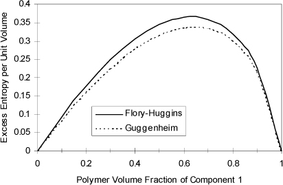
Figure 13.1. Excess entropy according to the Flory-Huggins equation versus Guggenheim’s equation at V2/V1 = 1695 for a polymer solvent mixture.
The Guggenheim form of the excess entropy is based on the molecular volume fractions, Φj, and the surface fractions, θj. Instead of using macroscopic property data to calculate volume fractions and surface fractions they are based on relative molecule volumes, r, and relative molecule surface areas, q, for each type of molecule.

The relative molecular parameters r and q may be calculated from group size and surface area parameters using the concept of group contributions. The size/area parameters are ratios to the equivalent size/area for the -CH2- group in a long chain alkane.11 The group parameters are added in the same manner as the UNIFAC method discussed in the next section and as given in Table 13.2 on page 512, except the UNIQUAC r and q values for alcohols are typically not calculated by group contributions (see the footnote to Table. 13.2). In the table, the uppercase Rk parameter is for the group volume, and the uppercase Qk parameter is for group surface area. From these values, the molecular size (rj) and shape (qj) parameters may be calculated by multiplying the group parameter by the number of times each group appears in the molecule, and summing over all the groups in the molecule,
Table 13.2. Selected Group Parameters for the UNIFAC and UNIQUAC Equationsa

a. AC in the table means aromatic carbon. The main groups serve as categories for similar subgroups as explained in the UNIFAC section.
b. Alcohols are usually treated in UNIQUAC without using the group contribution method. Accepted UNIQUAC values for the set of alcohols [MeOH, EtOH, 1-PrOH, 2-PrOH, 1-BuOH] are r = [1.4311, 2.1055, 2.7799, 2.7791, 3.4543], q = [1.4320, 1.9720, 2.5120, 2.5080, 3.0520]. See Gmehling, J., Oken, U. 1977-Vapor-Liquid Equilibrium Data Collection. Frankfort, Germany: DECHEMA.
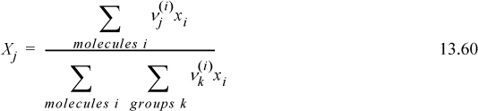
where ![]() is the number of groups of the kth type in molecule j. The subdivision of the molecule into groups is sometimes not obvious because there may appear to be more than one way to subdivide, but the conventions have been set forth in examples in the table and these conventions should be followed. The large number of possible functional groups is divided into main groups and further subdivided into structurally similar subgroups. Usually the functional groups include a nearest neighbor atom as part of the group. The group parameters are calculated from the van der Waals volume and van der Waals surface area. Note that the van der Waals volume and van der Waals area are not calculated from the van der Waals EOS. They are inferred from x-ray and other property data.12.
is the number of groups of the kth type in molecule j. The subdivision of the molecule into groups is sometimes not obvious because there may appear to be more than one way to subdivide, but the conventions have been set forth in examples in the table and these conventions should be followed. The large number of possible functional groups is divided into main groups and further subdivided into structurally similar subgroups. Usually the functional groups include a nearest neighbor atom as part of the group. The group parameters are calculated from the van der Waals volume and van der Waals surface area. Note that the van der Waals volume and van der Waals area are not calculated from the van der Waals EOS. They are inferred from x-ray and other property data.12.
Example 13.4. Combinatorial contribution to the activity coefficient
In polymer solutions, it is not uncommon for the solubility parameter of the polymer to nearly equal the solubility parameter of the solvent, but the mixture is still nonideal. To illustrate, consider the case when 1 g of benzene is added to 1 g of pentastyrene to form a solution. Estimate the activity coefficient of the benzene (B) in the pentastyrene (PS) if δps = δB = 9.2 and Vps and VB are estimated using group contributions. Use the Flory activity model and group contributions of UNIQUAC/UNIFAC to estimate volume fractions.
Since δps = δB = 9.2, we can ignore the residual contribution. Therefore,
Benzene is composed of 6(ACH) groups @ 0.5313 R-units per group ⇒ VB ∝ 3.1878. Pentastyrene is composed of 25(ACH) + 1(ACCH2) + 4(ACCH) + 4(CH2) + 1(CH3) ⇒ Vps ∝ 21.17:
Note: The volume fraction is close to the weight fraction because they are so structurally similar.
Flory’s model (no energetic contribution) predicts that the partial pressure of benzene in the vapor, yBP = xBγBPBsat, would be about 12% less than the ideal solution model.
The parameters to characterize the volume and surface area fractions have already been tabulated, so no more adjustable parameters are really introduced by writing it this way. The only real problem is that including all these group contributions into the formulas makes hand calculations extremely tedious. Fortunately, computers and spreadsheets make this task much simpler. As such, we can apply the UNIQUAC method almost as easily as the van Laar method.
For a binary mixture, the activity equations become

Like the Wilson equation, the UNIQUAC equation requires that two adjustable parameters be characterized from experimental data for each binary system. The inclusion of the excess entropy in UNIQUAC by Abrams et al. (1975) is more correct theoretically, but Wilson’s equation can be as accurate as the UNIQUAC method for many binary vapor-liquid systems, and much simpler to apply by hand. UNIQUAC supersedes the Wilson equation for describing liquid-liquid systems, however, because the Wilson equation is incapable of representing liquid-liquid equilibria as long as the λij parameters are held positive (as implied by their definition as exponentials, and noting that exponentials cannot take on negative values).
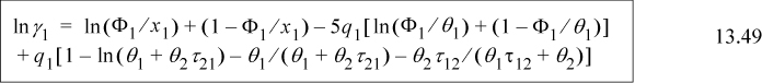
Extending Eqn. 13.40 to a multicomponent solution, the UNIQUAC equation becomes

Note that the leading sum is simply Flory’s equation. The first two terms are the combinatorial contribution and the last is the residual contribution. The parts can be individually differentiated to find the contributions to the activity coefficients,

13.5. UNIFAC
UNIFAC13 (short for UNIversal Functional Activity Coefficient model) is an extension of UNIQUAC with no user-adjustable parameters to fit to experimental data. Instead, all of the adjustable parameters have been characterized by the developers of the model based on group contributions that correlate the data in a very large database. The assumptions regarding coordination numbers, and so forth, are similar to the assumptions in UNIQUAC. The same strategy is applied:
The combinatorial term is therefore identical and given by Eqn. 13.54. The major difference between UNIFAC and UNIQUAC is that, for the residual term, UNIFAC considers interaction energies between functional groups (rather than the whole molecule). Interactions of functional groups are added to predict relative interaction energies of molecules. Examples are shown in Table 13.2. Each of the subgroups has a characteristic size and surface area; however, the energetic interactions are considered to be the same for all subgroups with a particular main group. Thus, representative interaction energies (aij) are tabulated for only the main functional groups, and it is implied that all subgroups will use the same energetic parameters. An illustrative sample of values for these interactions is given in Table 13.3. Full implementations of the UNIFAC method with large numbers of functional groups are typically available in chemical engineering process design software. A subset of the parameters is provided on the UNIFAC spreadsheet in the Actcoeff.xlsx spreadsheet included with the text. Knowing the values of these interaction energies permits estimation of the properties for a really impressive number of chemical solutions. The limitation is that we are not always entirely sure of the accuracy of these predictions.
Table 13.3. Selected VLE Interaction Energies aij for the UNIFAC Equation in Units of Kelvin

Although UNIFAC is closely related to UNIQUAC, keep in mind that there is no direct extension to a correlative equation like UNIQUAC. If you want to fit experimental data that might be on hand, you cannot do it within the defined framework of UNIFAC; UNIQUAC or NTRL is the preferred choice when adjustable parameters are desired. Although it is tedious to estimate the aij parameters of UNIQUAC or NRTL from UNIFAC, some implementations of chemical engineering process design software have included facilities for estimating UNIQUAC or NRTL parameters from UNIFAC. This approach can be useful for estimating interactions for a few binary pairs in a multicomponent mixture when most of the binary pairs are known from experimental data specific to those binary interactions.
The basic approach to understanding UNIFAC is the generalization of the methods for calculating the residual activity coefficient. Imagine the interactions of a CH3 group in a mixture of isopropanol (1) and component (2). The isopropanol consists of 2(CH3) + 1(CH) + 1(OH). Therefore, in the mixture, a CH3 will encounter CH3, CH, OH groups, and the groups of component (2), and the interaction energies depend on the number of each type of group available in the solution. Therefore, the interaction energy of CH3 groups can be calculated relative to a hypothetical solution of 100% CH3 groups. The mixture can be approximated as a solution of groups (SOG)14 (rather than a solution of molecules), and the interaction energies can be integrated with respect to temperature to arrive at chemical potential in a manner similar to the development of Eqn. 13.40.
Therefore, it is possible to calculate ![]() where
where ![]() is the chemical potential in a hypothetical solution of 100% CH3 groups and ΓCH3 is the activity coefficient of CH3 in the solution of groups. The chemical potential of CH3 groups in pure isopropanol (1), given by
is the chemical potential in a hypothetical solution of 100% CH3 groups and ΓCH3 is the activity coefficient of CH3 in the solution of groups. The chemical potential of CH3 groups in pure isopropanol (1), given by ![]() , will differ from
, will differ from ![]() because even in pure isopropanol CH3 will encounter a mixture of CH3, CH, and OH groups in the ratio that they appear in pure isopropanol, and therefore the activity coefficient of CH3 groups in pure isopropanol,
because even in pure isopropanol CH3 will encounter a mixture of CH3, CH, and OH groups in the ratio that they appear in pure isopropanol, and therefore the activity coefficient of CH3 groups in pure isopropanol, ![]() , is not unity, where the superscript (1) indicates pure component (1). The difference that is desired is the effect of mixing the CH3 groups in isopropanol with component (2), relative to pure isopropanol,
, is not unity, where the superscript (1) indicates pure component (1). The difference that is desired is the effect of mixing the CH3 groups in isopropanol with component (2), relative to pure isopropanol,
Fig. 13.2 provides an illustration of the differences that we seek to calculate, with water as a component (2).

Figure 13.2. Illustration relating the chemical potential of CH3 groups in pure 2-propanol, a real solution of groups where water is component (2), and a hypothetical solution of CH3 groups. The number of groups sketched in each circle is arbitrary and chosen to illustrate the types of groups present. The chemical potential change that we seek is ![]() . We calculate this difference by taking the difference between the other two paths.
. We calculate this difference by taking the difference between the other two paths.
If the chemical potential of a molecule consists of the sum of interactions of the groups,
Therefore, we arrive at the important result that is utilized in UNIFAC,

where the sum is over all function groups in molecule (1) and ![]() is the number of occurrences of group m in the molecule. The activity coefficient formula for any other molecular component can be found by substituting for (1) in Eqn. 13.56. Note that Γm is calculated in a solution of groups for all molecules in the mixture, whereas
is the number of occurrences of group m in the molecule. The activity coefficient formula for any other molecular component can be found by substituting for (1) in Eqn. 13.56. Note that Γm is calculated in a solution of groups for all molecules in the mixture, whereas ![]() is calculated in the solution of groups for just component (1). Note that we use uppercase letters to represent the group property analog of the molecular properties, with the following exceptions: Uppercase τ looks too much like T, so we substitute Ψ, and the aij for UNIFAC is understood to be a group property even though the same symbol is represented by a molecular property in UNIQUAC. The relations are shown in Table 13.4.
is calculated in the solution of groups for just component (1). Note that we use uppercase letters to represent the group property analog of the molecular properties, with the following exceptions: Uppercase τ looks too much like T, so we substitute Ψ, and the aij for UNIFAC is understood to be a group property even though the same symbol is represented by a molecular property in UNIQUAC. The relations are shown in Table 13.4.
Table 13.4. Comparison of Group Variables and Molecular Variables for UNIFAC

lnΓm is calculated by generalizing the UNIQUAC expression for ![]() . Generalizing Eqn. 13.55 and supporting equations,
. Generalizing Eqn. 13.55 and supporting equations,

where ![]() is the number of groups of type k in molecule i. Fortunately, the spreadsheet and programs provided with the textbook save us from doing the tedious calculations for UNIFAC, although an understanding of the principles is important.
is the number of groups of type k in molecule i. Fortunately, the spreadsheet and programs provided with the textbook save us from doing the tedious calculations for UNIFAC, although an understanding of the principles is important.
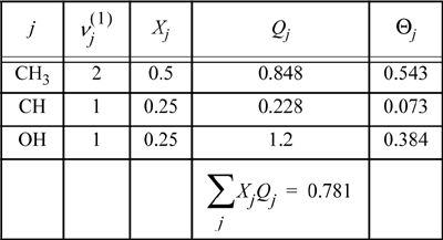
Example 13.5. Calculation of group mole fractions
Calculate the group mole fraction for CH3 in a mixture of 60 mole% 2-propanol, 40 mole% water.
Solution
The two molecules are illustrated in Example 13.1 on page 500 and the group assignments are tabulated there. On a basis of 10 moles of solution, there are six moles of 2-propanol, and four moles of H20. The table below summarizes the totals of the functional groups.

The mole fraction of CH3 groups is then XCH3 = 12/28 = 0.429. The mole fractions of the other groups are found analogously and are also summarized in the table. The results are consistent with Eqn. 13.60 which is more easily programmed,
Example 13.6. Detailed calculations of activity coefficients via UNIFAC
Let’s return to the example for the IPA + water system mentioned in Example 13.1. Compute the surface fractions, volume fractions, group interactions, and summations that go into the activity coefficients for this system at its azeotropic conditions. The isopropyl alcohol (IPA) + water (W) system is known to form an azeotrope at atmospheric pressure and 80.37°C (xW = 0.3146)a.
Applying Eqn. 13.57,
Solution
(this calculation can be followed interactively in the UNIFAC spreadsheet):
The molecular size and surface area parameters are found by applying Eqn. 13.44. Isopropanol has 2 CH3, 1 OH, and 1 CH group. The group parameters are taken from Table 13.2.
For IPA: r = 2·0.9011 + 0.4469 + 1.0 = 3.2491; q = 2·0.8480 + 0.2280 + 1.2 = 3.124 For water: r = 0.920; q = 1.40
At xW = 0.3146, ΦW = 0.1150, and θW = 0.1706 using the same combinatorial contribution as UNIQUAC, Eqn. 13.54,
Note that these combinatorial contributions are computed on the basis of the total molecule. This is because the space-filling properties are the same whether we consider the functional groups or the whole molecules.
For the residual term, we break the solution into a solution of groups. Then we compute the contribution to the activity coefficients arising from each of those groups. We have four functional groups altogether (2CH3, CH, OH, H2O). We will illustrate the concepts by calculating ![]() and simply tabulate the results for the remainder of the calculations since they are analogous.
and simply tabulate the results for the remainder of the calculations since they are analogous.
First, let us tabulate the energetic parameters we will need. We can summarize the calculations in tabular form as follows:

For pure isopropanol, we tabulate the mole fractions of functional groups, and calculate the surface fractions:
The same type of calculations can be repeated for the other functional groups. The calculation of ![]() is not necessary, since the whole water molecule is considered a functional group. Performing the calculations in the mixture, the mole fractions, Xj, need to be recalculated to reflect the compositions of groups in the overall mixture. Table 13.5 summarizes the calculations.
is not necessary, since the whole water molecule is considered a functional group. Performing the calculations in the mixture, the mole fractions, Xj, need to be recalculated to reflect the compositions of groups in the overall mixture. Table 13.5 summarizes the calculations.
Table 13.5. Summary of Calculations for Mixture of Isopropanol and Water at 80.37°C and xw = 0.3146
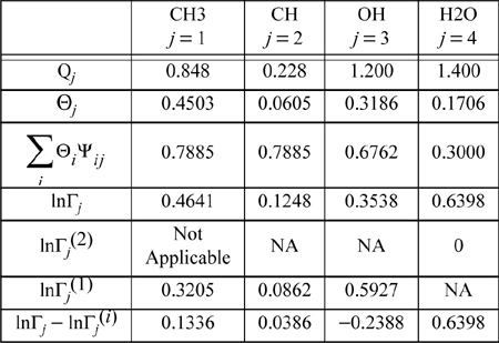
The pure component values of InΓj(i) can be easily verified on the spreadsheet after unhiding the columns with the intermediate calculations or in MATLAB by removing the appropriate “;”. Entering values of 0 and 1 for the respective molecular species mole fractions causes the values of InΓj(i) to be calculated. (Note that values will appear on the spreadsheet computed for infinite dilution activity coefficients of the groups which do not exist in the pure component limits, but these are not applicable to our calculation so we can ignore them.) Subtracting the appropriate pure component limits gives the final row in Table 13.5. All that remains is to combine the group contributions to form the molecules, and to add the residual part to the combinatorial part.
![]()
![]()
a. Perry, R.H., Chilton, C.H. 1973. Chemical Engineers’ Handbook, 5 ed. New York, NY: McGraw-Hill, Chapter 13.
13.6. COSMO-RS Methods
In principle, all electronic and molecular interactions are described by quantum mechanics, so you may wonder why we have not considered computing mixture properties from this fundamental approach. In practice, two considerations limit the feasibility of this approach. First, quantum mechanical computations tend to be time consuming. Precise computations can require days for a single molecule the size of naphthalene and the computation time increases as N7, where N is the number of atoms in the molecule. Second, the intermolecular interaction energy, which affects the mixing properties, is at least an order of magnitude smaller than the intramolecular energy. Therefore, high precision is required to compute the intermolecular interactions directly. Circumventing these limitations has been the focus of the “COSMO-RS” approach.
COSMO-RS is an abbreviation for “COnductor-like Screening MOdel for Real Solvents.” It refers to a method of performing quantum mechanical calculations as if the simulated molecule were in a conductive bath rather than a vacuum. The method was developed originally by Klamt and coworkers15 as an extension of previous work on a continuum solvation model (CSM).16 The implementation of Klamt and coworkers is marketed commercially as COSMOtherm and updated continually. A free educational version with graphical user interface is available that includes capability for about 350 compounds. The implementation of Klamt and coworkers is currently based on the TURBOMOLE package for quantum mechanical simulations, and a few other packages also provide consistent results. Later, Lin and Sandler developed an implementation based on the DMOL3 simulation package,17 which is included in the Accelrys Materials Studio. We refer to this implementation as COSMO-RS/SAC. It is available as a free download including capability for about 1500 compounds from a web site maintained by Y.A. Liu at Va. Tech.18 The method includes several empirical parameters that have been characterized by fitting experimental data. The specific parameters depend on the quantum simulation method. In the example below, we have applied the SAC parameters.
The key idea of the COSMO-RS approach has been to focus on the polarization of the surface surrounding a molecule. The significance of the surface polarization can be likened to the acidity and basicity of the SSCED model. If the surrounding surface is positively charged, then the molecular surface must be basic; if the surrounding surface is negatively charged, then the molecular surface must be acidic. If we imagine coloring these acidic interactions as blue and the basic interactions as red, we could represent the molecular surfaces in the manner of the pictures on the cover of the textbook. The overall surface energy, including positive, negative, and neutral influences, can be correlated with activity coefficients and other properties like the heat of vaporization.
To calculate the surface polarization an approximate quantum mechanical method can be applied, known as density functional theory (DFT). DFT computations typically require only a few hours for a molecule like naphthalene, and the increase in computation time scales as N3. If we integrate over the interactions between the surfaces of molecules, we can imagine how results similar to SSCED could be achieved. An additional advantage of COSMO-RS is that local composition effects are implicit in the integration of the local polarization interactions over all orientations between the two molecules. Furthermore, acidity and basicity are not limited to a single characteristic value per molecule, but are characterized by a range of polarizations over the entire surface of each molecule.
To implement the method, the molecular surface charges are calculated using DFT. The observed polarization is referred to as a σ-profile, where σ refers to the surface charge density (Coulombs/Å2). Typical σ-profiles are illustrated in Fig. 13.3. The p(σ) represents the amount of area per σ-interval (Å2/(Coulombs/Å2)) plotted against the surface charge density (Coulombs/Å2). In other words, p(σ) is proportional to a count of how many segments possess a given amount of surface polarization. It is analogous to the number of occurrences of a group in UNIFAC. The curve is normalized such that an integral of the σ-profile gives the total surface area of the molecule. The effective area per segment is divided out near the end of the calculation when computing the activity coefficient. The area under the curve in a particular region shows the total area of the molecule with the charge density. Fig. 13.3(a) shows how ethanol is a smaller molecule than octanol based on the total area under the curve.

Figure 13.3. Samples of σ-profiles for application to the COSMO-RS method, Aeffni(σ). Dashed vertical lines show the threshold values for hydrogen bonding.
Since the charge density, σ, ranges over negative and positive values, all values less than –0.0084 are considered to contribute to acidity. A similar consideration applies to the β contribution except that all σ > 0.0084 contribute to basicity. In Fig. 13.3(a), note that the two alcohols have extremely similar contributions of total area for both acidity and basicity. Fig. 13.3(b) shows that water is a very small molecule (small area under the curve) with extensive hydrogen bonding (both acidic and basic outside the dispersion bounds) while chloroform is a relatively large molecule with strong acidity and no basicity. All of these behaviors make sense qualitatively, so what remains is the translation into a quantitative method.
Computing activity coefficients for a binary solution is similar to the UNIFAC method if you can imagine transforming the earlier summation over groups to a summation over discretized polarization segments of the σ-profile. Note that use of the term “segment” does not refer to a geometric segment, but to an “interval” of surface polarization. A particular amount of surface polarization may occur at various places over the surface of the molecule, but all would be added together to get p(σ). It may be helpful to think of this quantity in mathematical terms rather than as a physical entity. Typically, the σ-profile is discretized into 51 values ranging from –0.025 to 0.025 (Coulombs/Å2).19 Therefore, we can refer to σk where k = [1,51]. To simplify the computations, the integration ∫p(σ)dσ ~ ΔσΣp(σk) is represented as a sum, Σp(k). The larger size of a particular molecule is reflected in the Σp(k) in a comparable manner to the molecular volume in the Scatchard-Hildebrand or SSCED models. Discretized segments on molecule i interact with segments on all molecules, including the ith molecule itself. In a mixture, pi(k) designates p(k) for the ith component. The activity coefficient contribution for a segment k(Γk) in a solution of polarization segments is analogous to Eqn. 13.57, but with a significantly different functional form.
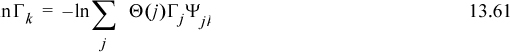
The surface area fraction of polarization segments in a binary mixture of molecules type 1 + 2 is

where ajk is defined below and the molecular surface area is
A practical difference between Eqns. 13.57 and 13.61 is that the activity coefficient contribution of a given σ-interval depends on itself through the summation over all interactions in Eqn. 13.61. Conceptually, the influence of a segment on its neighbors alters its own behavior as those neighbors respond to the local activity. This necessitates iteration, initiated with Γk = 1 for all k.
A fundamental difference between Eqns. 13.57 and 13.61 is that the formulas are derived entirely differently. The matrix of ajk is related to balancing electrostatic charges, as given by:
where α(j,k) and β(j,k) characterize the hydrogen bonding between the jth and kth segments, similar to the α and β parameters of the SSCED model. We assume that hydrogen bonding occurs regardless of which σ value (j or k) surpasses the threshold value because the energetic reward is sufficient for them to find each other regardless of where the segments are. Mathematically, this becomes,
Similar to UNIFAC, this approach leads to a nonunity value for the activity coefficient of a pure fluid. So,
where ![]() is computed using the same formula as for UNIFAC or UNIQUAC; Aeff = 7.5 is the normalization for the area, and Γk(i) is the segment activity in pure component i, computed by applying Eqn. 13.62 and so forth, with the appropriate composition.
is computed using the same formula as for UNIFAC or UNIQUAC; Aeff = 7.5 is the normalization for the area, and Γk(i) is the segment activity in pure component i, computed by applying Eqn. 13.62 and so forth, with the appropriate composition.
Although we can conceive of COSMO-RS as being similar to UNIFAC, it is really much more general. The UNIFAC method requires experimental data to characterize the aik matrix. COSMORS, on the other hand, computes this matrix based on σ-profiles that have been computed with no experimental data except the empirical constants in Eqn. 13.65. Usually, more precise results are obtained with UNIFAC if all the groups have been characterized, but the COSMO-RS approach can be used to supplement the UNIFAC method when no experimental data exist.
Example 13.7. Calculation of activity coefficients using COSMO-RS/SAC
σ-profiles for methanol and acetone are listed below. (a) Use these to compute the activity coefficient at xM = 0.425 and 55°C assuming the SAC values of the COSMO-RS parameters as given by Lin and Sandler. (b) Compute the activity coefficients over the entire range of compositions and compare to the fit of UNIQUAC to experimental data and the SSCED model.
Table of σ-profiles. Note that σ(k) = [-0.025,0.025], a total of 51 values. Cells omitted if all zeros.

Solution
a. Applying Eqn. 13.64 gives q1 = 67.9 and q2 = 102.6. The mixture’s segmental area fraction, Θ(k), is zero for k = 1 to 9. Θ(10)=(0.425(0.598) + (0.575)0)/(0.425(67.9) + (0.575)102.6) = 2.89(10-3) and so forth for Θ(11) to Θ(42).
For j = k = 1, σ(j) = σ(k) = –0.025. So, max(σ(j), σ(k)) = –0.025, and –0.025 – 0.0084 = – 0.0334, but max(0, –0.0334) = 0.
So α(1, 1) = 0, and even though β(1, 1) = –0.0166, the product α(1, 1)β(1, 1) =0 and hydrogen bonding contributes zero for i = k = 1. For the dispersion term, however,
a1,1 = [8233(σ(1) + σ(1))2]/0.001987 = 10359 and Ψ(1,1) = exp(–10359/328.15)=1.951(10–14).
The first term for which hydrogen bonding is nonzero is i = 1, k = 35. Then, α(1, 35) = max(σ(j), σ(k)) – 0.0084 = 0.0006 and β(1, 35) = –0.0166.
The total is a1,35 = [8233(–0.025 + 0.009)2 + 85580(0.0006)(–0.0166)]/0.001987= –428.98 and Ψ(1, 35) = exp(428.98/328.15) = 3.696. Note how p(k) contributes to Θ but not Ψ.
These two cases (i = k = 1) and (i = 1, k = 35) illustrate important behaviors. Briefly, segment pairs involving the disperse interactions between two like-charged segments are disfavored, as indicated by the small value of Ψ. Even when the polarizations are exactly opposite and sum to zero, the best that can happen for the dispersion term is Ψ = 1. All other values of polarization lead to Ψ<1 for the dispersion term (because the contribution is squared), reflecting an unfavorable interaction. This is vaguely reminiscent of the (Δδ’)2 term that applies to dispersion interactions in the SSCED model. The second case shows that acid-base interactions are opposite in sign to the dispersion interactions, and generally are sufficient to provide Ψ > 1, indicating favorable interactions. Again, this is reminiscent of hydrogen bonding in the SSCED model.
Completing the solution for part (a) involves summing all the terms, both for the mixture and for the pure fluid. After the first iteration of Eqn. 13.61 for Γk, the first 10 values are roughly 0.5. Other sample values are Γ20 = 1.561, Γ30 = 1.203, Γ40 = 0.736, and Γ50 = 0.500. After the last iteration, these values become Γ1 = 7.864(10–5), Γ10 = 0.0279, Γ20 = 1.478, Γ30 = 1.107, Γ40 = 2.522, Γ50 = 3.312(10–3).
Similarly, after the first iteration for pure fluids: Γk(1) = 0.5 for k = 1 to 10, ..., Γ20(1) = 1.559, Γ30(1) = 1.267, ... Γ1(2) = 0.501, Γ10(2) = 0.563, Γ20(2) = 1.562, and Γ30(2) = 1.176.
After the final iteration, Γ1(1) = 7.05(10–5), Γ10(1) = 2.931(10–2), Γ20(1) = 1.546, Γ30(1) = 1.204, ... Γ1(2) = 3.322(10–4), Γ10(2) = 3.748(10–3), Γ20(2) = 1.453, Γ30(2) = 1.063, ...
Summing the Γk – Γk(i) gives lnγ1 = 0.0957 – 0.0353 = 0.0605 and lnγ2 = 0.0746 – 0.0145 = 0.0601, where the negative terms are the Guggenheim-Staverman contribution using qi and r1 = 48.8 and r2 = 86.4. The values of r1 and r2 come from the (VT) database of Mullins et al.
b. The σ-profiles for methanol and acetone are shown below, along with a comparison to the activity coefficients from the SSCED model and the UNIQUAC model.a
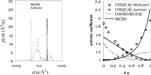
Regarding the σ-profiles, it is apparent from the high positive polarization (proton acceptor) of the acetone that hydrogen bonding should play a significant role. The right figure shows the comparison of the COSMO-RS model with a UNIQUAC fit (considered the benchmark in this case). The COSMO-RS/SAC model and the SSCED model are almost scaled mirror images, and neither is precisely correct.b The COSMO-RS/SAC model underestimates the nonideality of this mixture.
a. The UNIQUAC model (right figure) was fit to the data of Marinichev A.N., Susarev M.P. 1965. Zhur. Prikl. Khim, 38(2):371.
b. These components are available in the educational version of COSMOtherm. Estimates are more accurate with COSMOtherm, but the mirror-image effect is consistent.
13.7. The Molecular Basis of Solution Models
As discussed during the development of quadratic mixing rules, there comes a point at which the assumption of random mixing cannot completely explain the nonidealities of the solution. Local compositions are examples of nonrandomness. The popularity of local composition models like Wilson’s equation or UNIFAC means that we need to develop some appreciation of the strength of the underlying theory and its limitations. Similar to the situation for the random mixing models, there are limitations to the local composition models. At this time, however, we are not exactly sure what all the limitations are. This is still a question for active research. Nevertheless, we can provide an understanding of the assumptions in these models, because the assumptions are the sources of errors that impose limitations.
Extending the Energy Equation to Mixtures
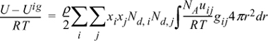
We begin the discussion with the energy equation, not the pressure equation as we did for pure fluids. This is because we are presently concerned with the Gibbs energy of mixing and its excess change relative to ideal solution behavior. It turns out that the excess Gibbs energy is dominated by the excess internal energy in most cases. In other words, the entropy of mixing is given with reasonable accuracy by the mixing rule on “b” given in Eqn. 12.1. Therefore, we focus our attention on extending the energy equation to mixtures. This requires revisiting our development of the energy equation for pure fluids and applying the same principles to extend it to mixtures. With two small modifications, the energy equation we developed for pure fluids becomes:

The small modifications are: (1) We have put the equation on an atomic basis instead of a molar basis by noting niNA = Ni and Nk = nR; (2) We recognize that these are the contributions to the energy departure that arise from atoms of type “1.” For the pure fluid, it so happens that we only have atoms of type “1.”
In developing the energy equation for pure fluids, we recognized that the average internal energy departure per atom [i.e., (U1 – U1ig)/N1] was equal to the energy per pair per unit volume times the local density in that volume integrated over the total volume. To make the extension to a mixture, we must simply recognize that there are now atoms of “type 2” around those atoms of “type 1.” To illustrate, consider a parking lot full of blue cars and green cars. If one parking lot had only green cars, then the average energy per green car would involve the average number of green cars at each distance around one green car times the energy associated with green cars being that distance from each other. If you pack them too close, you will have to work hard to pack them, and so forth. Now consider the next parking lot, where blue cars are mixed with green cars. The average energy per green car will now involve contributions from green-green interactions and blue-green interactions. In equation form, this becomes

We can check this equation by noting that it approaches the pure green car equation when all the blue cars leave the parking lot (i.e., as Nb → 0). We may next write the average energy per blue car by symmetry and the total energy by addition.

Finally, making the substitutions in terms of the mole fractions, recognizing that ubg=ugb and gbg=ggb, and converting back to a molar basis, we see that for multicomponent mixtures,
Comparing to the van der Waals equation for pure fluids,

where ![]() and it is understood that aij = aji.
and it is understood that aij = aji.
In this form we can recognize that the radial distribution functions may be dependent on composition as well as temperature and density. Therefore, assuming the quadratic mixing rule simply neglects the composition dependence of the a parameter, as well as the temperature and density dependence. We found in Unit II that the assumptions about temperature and density in the van der Waals equation were flawed and that is what motivated the Peng-Robinson equation. Similarly, neglecting the composition dependence of the radial distribution functions leads to some limitations that give rise to local composition theory.
Local Compositions in Terms of Radial Distribution Functions
Recalling the energy equation for mixtures, Eqn. 13.71 multiplied by RT,

We may now define the local compositions in terms of the radial distribution functions.
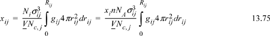
where rij = r / σij
Rij = “neighborhood”
Nc,i = total # of atoms around sites of type “i,” that is, the coordination number.
Rearrangement gives the molecular definition of the local composition parameter Ωij,

and we note the similarity between the integral in the energy equation and the integral in the definition of local composition.
For a square-well fluid, εij = constant, so we can factor it out of the integral,

Substituting Nc,j, and xij into the energy equation for mixtures (multiply Eqn. 13.75 by Nc,j and substitute into Eqn. 13.78),
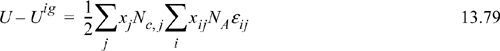
This is the equation previously applied as the starting point for development of the Gibbs excess energy model from a local composition perspective. The rest of the derivation proceeds as before.
Assumptions in Local Composition Models
In the previous section, we discussed some of the currently popular expressions for activity coefficients. We listed the assumptions involved in developing the expressions but we did not take time to discuss those assumptions. Instead, we directly applied the expressions as a practical necessity and moved on. In this section, we recall those assumptions and attempt to put them in perspective. After developing this perspective, we conclude with a word of caution; the reliability of the predictions depends largely on the accuracy of the assumptions.
The local composition theory, upon which UNIQUAC and others are based, has the general intent of correcting regular solution theory for asymmetries in solution behavior due to fluid structure near a central species. Relaxing the assumption that SE = 0 also leads to the necessity of considering the entropy of mixing, and differences between the UNIQUAC model and Wilson’s model are primarily due to differences in treatment of SE. In review, four assumptions are shared by the local composition theories when considered with respect to spheres:
1. The average energy of an i-j interaction is independent of temperature, density, and other species present.
2. (A – Ais) = (G – Gis).
3. The “coordination number” of a specie in a mixture is the same as that of the pure species.
4. The temperature-dependent part of the energy of mixing is given by Ωij = (σij/σij)3 exp[z(εij – εjj)/2kT] where z is a “coordination number.”
Wilson’s equation makes the following assumptions:
5w. Nc,j = z = 2 for all j at all densities.
6w. ![]() .
.
7w. (σij/σjj)3 = Vi/Vj for all i, j, and ![]() , Λji = Ωij.20
, Λji = Ωij.20
UNIFAC(QUAC) makes the following assumptions:
![]()
![]()
7u. (σij/σjj)3 = Nc,i/Nc,j = qi/qj for all i, j, ![]() .
.
Assumption 1 involves factoring some average energy out of the energy integral such that the local composition integral is obtained. As noted, this assumption would be correct for a square-well potential, so we can probably trust that it would be reasonable for other similar potentials like the Lennard-Jones. The doubt which arises, however, involves the application of this approximation to highly nonideal mixtures. The square-well and Lennard-Jones potentials rarely give rise to highly nonideal mixtures when realistic values for their parameters are chosen. There is very little evidence to judge whether the εij factored out in this way is really independent of temperature and density for nonideal mixtures. In fact, in Chapter 1, we showed that dipole interactions are temperature dependent.
Assumption 2 has to do with neglecting ln(Z/Zis). For liquids, this may seem dangerous until one realizes that it amounts to neglecting ln(1 + ρE/ρ) ≈ ρE/ρ. Relative to the density of a liquid, the excess density is generally small (but easy to measure with a high degree of accuracy) and this assumption is acceptable.
Assumption 3 has to do with convenience. If the coordination number of each species was assumed to change with mixing, the theory could become very complicated. That is not a very good physical reason, of course. Physically speaking, this assumption could become quite poor if the sizes of the molecules (or segments in the case of UNIFAC) were very different.
Assumption 4 is the primary assumption behind all of the current local composition approaches, but it is not required by the concept of local compositions. It is simply computationally expedient in the equations that develop. The crucial aspect of the assumption is the simple form of the temperature dependence of Ωij. The main motivation for this assumption appears to be obtaining an expression which can be integrated analytically. But how accurate is this assumption on a physical basis? Moreover, how can we determine the physical behavior for the behavior of Ωij in an unequivocal manner? Merely fitting experimental data for the Gibbs excess function is equivocal because some set of adjustable parameters will provide a good fit even if the model has no physical basis. An alternative available to us that was not available to van der Waals is to apply computer simulation of square-well mixtures over a specific range of densities and temperatures and test the validity of Wilson’s approximation directly through the simulated local compositions. This approach was undertaken by Sandler and Lee.21
Sandler and Lee have developed a correlation for what amounts to Ωij of a square-well potential.

This expression reproduces the local compositions of a substantial set of molecular simulation data which Sandler and coworkers have generated. We can therefore use this expression along with the molecular simulation data as a guide to the accuracy of Wilson’s assumption.
The most important consideration is the temperature dependence of this parameter because it is the integration with respect to temperature that allows us to get from energy to free energy. As for density, it could be argued that the density of all liquids is roughly the same, so it is not unreasonable to pick a specific density and just study the temperature effects. Suppose
If the natural logarithm term on the right-hand side in the above equation is small or gives rise to a contribution which is linear in 1/kT, then Wilson’s assumption is basically correct and his definition of εij would just be a little different from Eqn. 13.18. If ln Ωij versus 1/kT is not linear, however, then Wilson’s assumption is very questionable. Fig. 13.4 shows ln Ωij is fairly linear over certain ranges of temperature. This suggests that the primary assumption of Wilson and UNIFAC(QUAC) is not unreasonable. Does this mean that the problem of nonideal solutions is solved? Maybe, but maybe not. Unfortunately, we must look closely at the range of temperatures that are applicable. This range is limited by the tendency for the mixture to phase-separate. That is, dropping the temperature at constant overall density eventually places the conditions inside the binodal curve. For the composition and density listed above, the binodal occurs when NA(ε12 – ε12)/RT < –0.4. This corresponds to a maximum value of A12 in Wilson’s equation on the order of ~300 cal/mol at temperatures near 400 K. To use larger values for A12 would be unsupported, but larger values are often used, as illustrated in Example 13.3.

Figure 13.4. Temperature-dependence of local composition parameters. Points are molecular simulation data and the curve is the correlation of Sandler and Lee.21 The approximate linearity of the plot lends support to the assumption applied in integrating the internal energy to obtain the free energy.
Another indication of the potential for error with the local composition approach is given by experimental data for excess enthalpies of mixing. Relations from classical thermodynamics make it possible to estimate the enthalpy of mixing by taking the derivative of the Gibbs energy of mixing with respect to temperature. Larsen et al., have developed a modified form of UNIFAC to address this problem.22 Not surprisingly, the modification involves the introduction of a substantial number of additional adjustable parameters. Even though the modified form does improve the accuracy of all the thermodynamic properties for a large number of systems there are many systems for which the predicted heats of mixing are in error by 100%–700%. More importantly, there is no way of knowing in advance when the predictions will be in error or when they will be accurate.
So why do these approximations fit the activity coefficient data? Because they have enough adjustable parameters to fit the data. Even the Margules one-parameter equation is good enough for that in many cases, but we suffer few delusions about its physical accuracy. In conclusion, we must say that local composition theory has much to recommend it. It does fit a great wealth of experimental data and there is some justification for its form via the theoretical physics which can be applied. But it is often extrapolated too far and that can lead to miscalculations by unwary users. In the end, we must never underestimate the value of experimental data for nonideal mixtures and apply the currently available theory with a careful and mildly critical view.
Assumptions 5 through 7 have to do with the entropy of mixing. The inclusion of the Staverman-type modifications to address the differences between surface fraction and volume fraction are generally recognized to be reasonable based on polymer lattice computer simulations. This modification and the estimate of molecular volumes by group contributions instead of liquid molar volumes comprise the primary differences between the Wilson and UNIQUAC models.
The UNIFAC theory is distinguished from UNIQUAC in that the solution is assumed to be a mixture of functional groups, not molecules. The UNIQUAC theory is then applied to each type of group interaction. The values for the group interactions are then regressed from a data base that includes phase equilibrium data for many, many systems. In one sense, the UNIFAC method is more like a massive regression than a truly predictive method. Thus, it lies somewhere between the purely correlative method of fitting van Laar constants and the purely predictive method of the Scatchard-Hildebrand theory (or any equation of state with kij = 0). Like any regressed equation, it can be unreliable if extrapolated far beyond the originally applied data. If you are ever in the position of designing truly novel chemical systems, you should be especially sensitive to the need for specific experimental data.
13.8. Summary
The theories developed in this chapter are based on the local composition concept. Similar to models developed in the previous chapter, accurate representation of highly nonideal solutions requires the introduction of at least two adjustable parameters. These adjustable parameters permit us to compensate for our ignorance in a systematic fashion. By determining reasonable values for the parameters from experimental data, we can interpolate between several measurements, and in some cases extrapolate to systems where we have no measurements. Learning how to determine reasonable values for the parameters and apply the final equations is an important part of this chapter. We also introduce the UNIFAC model, which is useful for predicting behavior when no experimental measurements are available. Similar to UNIFAC, COSMO-RS methods are predictive, but are based on quantum mechanical simulations that can be applied when experimental data are entirely lacking for a particular functional group. UNIFAC would require at least a small quantity of experimental data to characterize the group contributions.
We should also note, however, that using an equation of state is similarly simplified by using a computer, so the basic motivation for developing solution models specific to liquids is simultaneously undermined by requiring computers for implementation. From this perspective, what we should be doing is analyzing the mixing rules and models of interaction energies in equations of state if we intend to use a computer anyway. We return to this point in Unit IV, when we discuss hydrogen-bonding equations of state for nonideal solutions.
13.9. Important Equations
The UNIFAC method receives broad application throughout thermodynamic modeling. In fact, occasional applications of UNIFAC may be too broad in the sense that experimental data specific to a particular binary system are ignored and UNIFAC predictions are not validated with actual measurements. A literature search should be conducted for experimental data pertaining to every molecular interaction in a mixture and compared to the UNIFAC predictions. If significant deviations are observed, then UNIQUAC (or Wilson or NRTL) should be applied as the general activity model with system-specific parameters whenever possible and parameters inferred from UNIFAC predictions only in cases where no experimental data are available. In that context, an important equation for this chapter is best characterized by the UNIQUAC model.
Fundamentally, the energy equation for mixtures summarizes all local composition models:
13.10. Practice Problems
P13.1. The following lattice contains x’s, o’s, and void spaces. The coordination number of each cell is 8. Estimate the local composition (Xxo) and the parameter Ωox based on rows and columns away from the edges. (ANS. 0.68,1.47)
13.11. Homework Problems
13.1. Show that Wilson’s equation reduces to Flory’s equation when Aij = Aji = 0. Further, show that it reduces to an ideal solution if the energy parameters are zero, and the molecules are the same size.
13.2. The actone(1) + chloroform(2) system has an azeotrope at x1 = 0.38, 248 mmHg, and 35.17°C. Fit the Wilson equation, and predict the P-x-y diagram.
13.3. Model the behavior of ethanol(1) + toluene(2) at 55°C using the UNIQUAC equation and the parameters r1 = 2.1055, r2 = 3.9228, q1 = 1.972, q2 = 2.968, a12 = –76.1573 K, and a21 = 438.005 K.
13.4. The UNIFAC and UNIQUAC equations use surface fraction and volume fractions. This problem explores the differences.
a. Calculate the surface area and volume for a cylinder of diameter d = 1.0 and length L = 5 where the units are arbitrary. Calculate the surface area for a sphere of the same volume. Which object has a higher surface area to volume ratio?
b. Calculate the volume fractions and surface area fractions for an equimolar mixture of the cylinders and spheres from part (a). Use subscript s to denote spheres and subscript c to denote cylinders.
c. For this equimolar mixture, calculate the local composition ratios xcs/xss and xsc/xcc for the UNIQUAC equation if the energy variables τcs and τsc are unity. For the equimolar mixture, substitute the values of volume fraction and surface fraction into the expression for UNIQUAC activity coefficients, and simplify as much as possible, leaving the q’s as unknowns.
d. Consider n-pentane and 2,2-dimethyl propane (also known as neopentane). Calculate the UNIQUAC r and q values for each molecule using group contribution methods. Compare the results with part (a). [Hint: You might want to think about the -C-C-C-bond angles.]
13.5. Consider a mixture of isobutene(1) + butane(2). Consider a portion of the calculations that would need to be performed by UNIFAC or UNIQUAC.
a. Calculate the surface area and volume parameters for each molecule.
b. Provide reasoning to identify which component has a larger liquid molar volume. Which compound has a larger surface area?
c. Calculate the volume fractions for an equimolar mixture.
13.6. Solve problem 10.14 using UNIFAC to model the liquid phase.
13.7. The flash point of liquid mixtures is discussed in Section 10.5. For the following mixtures, estimate the flash point temperature of the following components and their equimolar mixtures using UNIFAC:
a. methanol (LFL = 7.3%) + 2-butanone (LFL = 1.8%)
b. ethanol (LFL = 4.3%) + 2-butanone (LFL = 1.8%).
13.8. Use the UNIFAC model to predict the VLE behavior of the n-pentane(1) + acetone(2) system at 1 bar and compare to the experimental data in problem 11.11.
13.9. According to Gmehling et al. (1994),23 the system acetone + water shows azeotropes at: (1) 2793 mmHg, 95.1 mol% acetone, and 100°C; and (2) 5155 mmHg, 88.4 mol% acetone and 124°C. What azeotropic pressures and compositions does UNIFAC indicate at 100°C and 124°C? Othmer et al. (1946) (cf. Gmehling24) have studied this system at 2570 mmHg. Prepare T-x-y or P-x-y plots comparing the UNIFAC predictions to the experimental data.
13.10. Consider the experimental data of Brown and Smith (1954) cited in problem 10.2. Prepare a P-x-y plot and a plot of experimental activity coefficients vs. composition. Then use UNIFAC to predict the activity coefficients across the composition range and add the calculations to the plots.
13.11. Flash separations are fundamental to any process separation train. A full steady-state process simulation consists largely of many consecutive flash calculations. Use UNIFAC to determine the temperature at which 20 mol% will be vaporized at 760 mmHg of an equimolar mixture liquid feed of n-pentane and acetone.
13.12. A preliminary evaluation of a new process concept has produced a waste stream of the composition given below. It is desired to reduce the waste stream to 10% of its original mass while recovering essentially pure water from the other stream. Since the solution is very dilute, we can use a simple equation known as Henry’s law to represent the system. According to Henry’s law, ![]() . Use UNIFAC to estimate the Henry’s law constants when UNIFAC parameters are available. Use the Scatchard-Hildebrand theory when UNIFAC parameters are not available. Estimate the relative volatilities (relative to water) of each component. Relative volatilities are defined in problem 11.2.
. Use UNIFAC to estimate the Henry’s law constants when UNIFAC parameters are available. Use the Scatchard-Hildebrand theory when UNIFAC parameters are not available. Estimate the relative volatilities (relative to water) of each component. Relative volatilities are defined in problem 11.2.
Compositions in mg/liter are:

13.13. Derive the form of the excess enthalpy predicted by Wilson’s equation assuming that Aij’s and ratios of molar volumes are temperature-independent.
13.14. Orbey and Sandler (1995. Ind. Eng. Chem. Res. 34:4351.) have proposed a correction term to be added to the excess Gibbs energy of mixing given by UNIQUAC. To a reasonable degree of accuracy the new term can be written
where
Derive an expression for the correction to the activity coefficient. [Hint: Do you remember how to differentiate implicitly?]
13.15. The energy equation for mixtures can be written for polymers in the form:
By analogy to the development of the Scatchard-Hildebrand theory, this can be rearranged to:
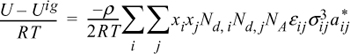
where
Nd,i = degree of polymerization for the ith component
ρ = molar density
xi = mole fraction of the ith component
NA = Avogadro’s number
U = molar internal energy.
aii* = 3 + 2/Ndi
aij* = (aii* ajj*)1/2
![]()
εij = (εii εjj)1/2
Derive an expression for lnγ1 for the activity coefficient model presented above.
13.16. Use the UNIFAC model to predict P-x-y data at 90°C and x1, = {0, 0.1, 0.3, 0.5, 0.7, 0.9, 1.0} for propanoic acid + water. Fit the UNIQUAC model to the predicted P-x-y data and report your UNIQUAC a12 and a21 parameters in kJ/mole.
a. Rearrange Eqn. 13.22 to obtain Eqn. 13.23.
b. Use Eqns. 13.16 and 13.18 in Eqn. 13.17 and perform the integration to obtain Eqn. 13.19.
c. Use Eqns. 13.16 and 13.31 in Eqn. 13.17 and perform the integration to obtain Eqn. 13.40.
13.18. Fit the data from problem 11.11 to the following model by regression over all points, and compare with the experimental data on the same plot, using the
a. Wilson equation
b. NRTL equation
c. UNIQUAC equation
13.19. Work problem 11.25 using the
a. Wilson equation
b. NRTL equation
c. UNIQUAC equation
13.20. Work problem 11.26 using the
a. Wilson equation
b. NRTL equation
c. UNIQUAC equation
13.21. Using the data from problem 11.27, fit the specified model equation and then plot the P-x-y diagram at 80°C using the
a. Wilson equation
b. NRTL equation
c. UNIQUAC equation