Estimating Volatilities

I can observe an asset's return; it is the percentage change in the observed market value of the asset between two well-defined points in time. Strictly speaking, I cannot observe the volatility of the return. I can only estimate it. In Chapter 5, volatility—or standard deviation—was a sample statistic. It was the square root of the return variance. The variance was the mean of the squared deviations of returns from their sample mean. We didn't discuss N—the sample size. The implicit assumption was that N was the size of the historical example. As statisticians, we prefer N to be large, as more information is preferred to less when estimating statistics. The annualized volatility of the return on the S&P 500 since 1950 is 14.7 percent. That is a volatility averaged over 60 years (N = 721). But what if I think that the market today is not average, that is, what if the market is clearly in a high or low volatility regime?

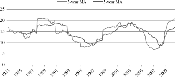
Analysts use several cheap methods to deal with changing volatility. One method is to measure volatility over a short trailing horizon as a moving average, for example, using a trailing three-year or five-year window. The choice of window width is arbitrary but the idea is to provide a long enough window to generate meaningful estimates while at the same time trying to keep the window short enough to capture the present volatility regime. This method is clearly suboptimal for three reasons: first, it throws away data outside the window while the moving average process creates a highly correlated series. Second, it still gives all the data equal weight. If the point was to give more recent observations greater weight, then this method doesn't really work. Analysts then roll this window forward as well, so that in each period, the volatility is reestimated, creating, in effect, a highly correlated time series of volatilities. Using a 36-month rolling window will create a time series of monthly volatilities for which adjacent volatility estimates have 35 observations in common in their respective samples. And third, if there is a regime shift in volatility, this method will not incorporate it for some time to come. Figure 11.4 shows the volatility cycling of the S&P 500 using both three-year and five-year windows.

Figure 11.4 S&P 500 Volatility

The five-year moving average (MA) provides more smoothing since the series is being averaged over a longer period of time. Higher volatility regimes should be obvious surrounding the crash of October 1987, the default of Long-Term Capital Management in 1989, the tech bubble crash in 2001, and the credit crisis beginning in 2008. Clearly, assuming volatility is equal to a constant long-term average of 14.7 percent would appear too restrictive as volatility obviously has time series properties that we would like to exploit.

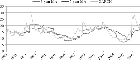
Figure 11.5 imposes the GARCH(1,1) volatility estimate (I use a GARCH(1,1) process that I derive further on) on top of these two MA estimates using S&P 500 price returns from 1980 to the present. I will provide an intuitive derivation of GARCH in a moment, but to fix ideas, I think it is interesting to contrast this maximum likelihood volatility estimator to the three- and five-year MA estimators. I mentioned earlier that the MA would lag volatility developments in the market. Take the 2008 credit crisis, for example. The five-year MA volatility estimate relies on equal weighting of the trailing 60 months of return, that is, it smoothes the impact of more recent events across this longer time horizon. We see quite clearly that it is underestimating what true volatility must surely be to the extent that its volatility estimate has barely budged above the long-term unconditional mean volatility of 14.7 percent. The same is true for the three-year MA estimate but more muted since it is smoothing returns over a shorter trailing 36-month period. The GARCH estimate, on the other hand, is much more responsive, showing a sharp spike up in risk at the beginning of the crisis in 2008.

Figure 11.5 S&P 500 Volatility

Smoothed MA estimates of volatility also have the property of creating a memory where none is deserved. Notice, for example, that both MA volatilities remain artificially high after the crash of October 1987 as well as the 2001 tech bubble crash. In contrast, the GARCH estimate recovers from these transitory shocks more quickly. And while GARCH volatility estimates have come down in 2010 (consistent with other market measures of risk like the VIX), the MA estimators will remain artificially high for some time to come.

These are clearly undesirable properties—MA estimators use less information, treat the distant past as if it were as important as the present, and produce biased forecasts. One response to simple MA estimators is to use all of the available data (instead of a moving window) and weight observations so that more recent returns have higher weight. These are still moving averages, but they are exponentially weighted so that the most recent observation has a weight of one and weights decline exponentially to zero (but not exactly zero) into the past. This has a certain intuitive appeal. I will develop this idea now and use it to derive the GARCH estimator.

As in Chapter 1, we define the one-period return to an asset as:

Assuming a sample size of m, then a consistent estimator—this is the maximum likelihood estimator—for the return variance is

Notice that the weight 1/m is equal for all observations and that the sum of the weights is one. With no loss of generality, assume the mean return is zero and allow for the weights to vary across time but still sum to one as in:

We will focus now on the weights α_i. First, let's assume further that the variance has a long run mean β₀, and add this to the process:

Finally, assume that the weights exponentially decline according to (0 < λ < 1):

Making this substitution gives us the exponentially weighted moving average (EWMA):

The weights αλ^i–1 are time dependent with decay parameter λ. A word on exponential weighting is in order here. If we wanted to construct an exponentially weighted series of returns, for example, we would need to choose a value for λ. One way to do this is to think of a half-life, that is, the point in time going back in the sample for which that observation has a weight equal to 0.5. If we set, for example, a half-life of 36 months, then what we are imposing is that the return at that point has half the weight of the current return (and exponentially continues to decay thereafter toward zero). More explicitly, we seek a value for the decay rate, in this case, such that, in general, λ^t = 0.5. Taking natural logarithms on each side gives us:

Therefore, given a value for t, say, 36 months, we solve for λ, which in this case is 0.992. Substituting this parameter into the preceding equation provides the required weight decay pattern.

There are two problems with EWMA. The first and more obvious concerns the arbitrary choice of half-life, which is subjective. We will return to this point in a moment. The second problem is subtler; it has to do with the properties of the EWMA variance model. In particular, this model of volatility is not mean-reverting. That means that we are not guaranteed that the volatility process will return to a long-run equilibrium and, in fact, it could be nonstationary. In a word, nonstationary means that the mean and variance (and higher moments) of the returns series are functions of time. A random walk is one such example. Properties of nonstationary series include inconsistent test statistics (the usual t and F statistics). In many cases, first differences generate stationarity. For econometricians, this is a hugely significant weakness to the model. Fortunately, GARCH shares none of these weaknesses, and in fact, the EWMA can be shown to be a special case of GARCH. Let me try to develop the GARCH intuition from the EWMA model.

Once again, let's simplify whenever possible. First, we will assume that the long-run mean variance β₀ is zero and that α = 1. Now, we can focus on the decay parameter. We have the following:

If we then expand the resulting variance specification by writing the summation out, we get:

Lagging this one period gets us the following:

Now, multiply this last equation by λ on both sides:

subtract it from the previous equation, and simplify to get:

This is basically the result we want, but this can be simplified further because the last term goes to zero as m gets large, that is,

If we restrict the weights on the two remaining terms to sum to one, then we can write our new variance formula as follows:

Those of you who have studied time series analysis recognize this as the GARCH(1,1) process. It has one autoregressive component and one moving average component,. The final specification, which includes the long-run mean variance is specified as:

where (α+β) < 1 for stationarity and (β₀ + α + β) = 1. Estimation is by maximum likelihood. Most software packages return estimates for α, β, and the long-run mean V_L. What is especially attractive is that the decay parameters is a maximum likelihood estimate and therefore optimal. I have found that during the crisis beginning in 2008, GARCH(1,1) estimates of the half-life are much shorter than those used by EWMA and that these parameters can be quite variable over time.

The GARCH(1,1) estimates that were presented in the preceding graphic for the S&P 500 can be found on the Chapter 11 spreadsheet. This specification is convenient since it provides a one-step ahead forecast for the volatility of the series. That is, the current forecast is computed given values for the lagged volatility and last period's squared return deviation, and the maximum likelihood parameter values. Forecasts for t + k can be derived by recursive substitution. For example, the k-step ahead forecast is a function of the t + 1 through t + k – 1 forecasts. Most software packages that estimate GARCH volatilities also have commands available for out-of-sample forecasts.