Pricing European Call Options
Let's use the idea of a replicating portfolio to derive the value of a call option. We'll begin with a single period problem depicted in Figure 16.5. Think of a stock whose spot price S can go up at the end of one period by a factor u to the level uS or can go down by a factor d to dS. I will derive the parameters u and d in Chapter 17. Moreover, suppose that the return on a risk-free loan is ![]() . Thus, we have the payout shown in Figure 16.5.
. Thus, we have the payout shown in Figure 16.5.
Figure 16.5 Single Period Payout Space

The call option will have the payout space given in Figure 16.6.
Figure 16.6 Call Payout Space

We want to use a combination of an investment in the stock and the risk-free asset to mimic the value of the call option. Letting Cu and Cd stand for the value of the call should the stock price rise or fall, respectively, then our aim is construct a riskless portfolio consisting of a long position of $x in the stock and $b in the risk-free asset plus a short position in one call option. If stock prices rise, we get the first of the following two equations; if they fall, we get the second equation. No arbitrage means that these will hold (otherwise, we can profit with no risk by selling calls in exchange for stock and vice versa). The question is how much of the stock do we need (x) and how much do we lend (b)? Thus, we solve the following for x and b:
![]()
We can solve the following system for x and b:
![]()
This has the solution given by:
![]()
Therefore, the replicating portfolio is the sum:
![]()
Substituting ![]() and recognizing that
and recognizing that ![]() simplifies this as:
simplifies this as:
![]()
Finally, realizing that ![]() must equal the value of the call, we immediately have the result:
must equal the value of the call, we immediately have the result:
![]()
Here the parameter q plays the role of a probability in determining the expected value. This says that the current period value of the call option is the discounted expected value of the next period valuations (see Figures 16.5 and 16.6). Notice that q does not include the stock's expected return and this feature is what makes this risk-neutral pricing because it does not depend in any way on our preferences toward risk. This is our major result. As an example, take the case of a one-month call option with current underlying share price ![]() and a strike price
and a strike price ![]() . Note that the option is currently in the money. Assume that the annual risk-free rate is 10 percent, implying that the monthly risk-free rate return is
. Note that the option is currently in the money. Assume that the annual risk-free rate is 10 percent, implying that the monthly risk-free rate return is ![]() and let's assume the up and down movement multipliers are
and let's assume the up and down movement multipliers are ![]() and
and ![]() . From these values, we solve
. From these values, we solve ![]() . Figure 16.7 illustrates the possible share prices one month out along with the call option values. Let's discuss how these numbers were arrived at.
. Figure 16.7 illustrates the possible share prices one month out along with the call option values. Let's discuss how these numbers were arrived at.
Figure 16.7 One-Period Call Option on a Stock

It's easy to see how the two share prices are arrived at. ![]() and
and ![]() . The call option values corresponding to these two prices are derived from
. The call option values corresponding to these two prices are derived from ![]() . If the share price rises to $1.06, then the call has value
. If the share price rises to $1.06, then the call has value ![]() . Otherwise, if the share price falls to $0.94, the call has value $0.04. The value of the call presently is a weighted average of these two terminal call option values with weights q and
. Otherwise, if the share price falls to $0.94, the call has value $0.04. The value of the call presently is a weighted average of these two terminal call option values with weights q and ![]() . This gives us:
. This gives us:
![]()
This says that the fair price for the option to buy a currently priced $1 share of stock one month from now for $0.9 is 11 cents. A multiple-period model of stock prices is a natural extension, which we see in Figure 16.8.
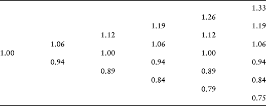
Figure 16.8 Multiperiod Price Lattice

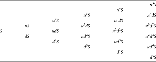
Figure 16.9 Multiperiod Stock Dynamic

![]()
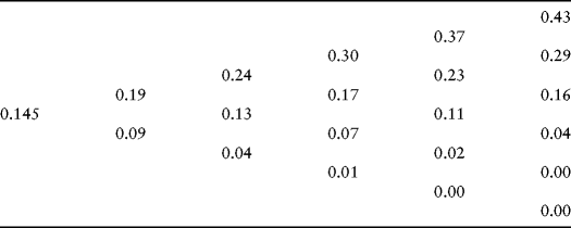
Figure 16.10 Call Option Value


![]() Go to the companion website for more details.
Go to the companion website for more details.
