
The Greek Letters
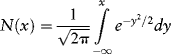
Let's now take a closer look at this model. First, let us define the cumulative standard normal distribution function because we are going to need this to evaluate Black-Scholes:
N(x) is bounded between zero and one since it is a probability. Thus, N(d1) for example, substitutes d1 for x in this expression and is increasing in the value of d1 which, itself, is a positive function of the difference between the current spot price S0 and the strike price K as well as the risk-free return but is negatively related to the underlying volatility. From the definitions given earlier, it follows that d2 is also declining in volatility. It is easy to demonstrate using a spreadsheet that both N(d1) and N(d2) are declining in volatility but that their spread is increasing in volatility and this proves that the value of the call option will rise with volatility. The intuition here is that as volatility rises, so does the likelihood that the option will be in the money. This, actually, is the notion of the option's vega—its sensitivity to underlying volatility.
These initial observations give rise to a host of questions regarding the sensitivity of the call option value to changes in the underlying parameters. These questions involve solving for the so-called Greek letters, a topic to which we now turn our attention. I will demonstrate these for the call option. Extension to put options is straightforward.
The first question of interest asks how sensitive the call option's value is to movements in the underlying spot price. This is called the option's delta, specifically, ![]() The delta is therefore bounded like a probability—it is the cumulative standard normal density evaluated at d1. From the discussion just had, it is going to be higher (lower) the lower (higher) is the volatility on the underlying security's return. Low volatility stocks, for example, are going to have a relatively higher delta because movements in price of any size are expected to be less likely than for higher volatility stocks. Thus, call value on lower volatility stocks is more sensitive to changes in spot prices. At the same time, delta responds to the relationship between spot and strike prices, moving higher as the option displays more moneyness (S > K) and vice versa. This result is also intuitive; option value is not going to be very sensitive to changes in price if the option is out of the money (OTM).
The delta is therefore bounded like a probability—it is the cumulative standard normal density evaluated at d1. From the discussion just had, it is going to be higher (lower) the lower (higher) is the volatility on the underlying security's return. Low volatility stocks, for example, are going to have a relatively higher delta because movements in price of any size are expected to be less likely than for higher volatility stocks. Thus, call value on lower volatility stocks is more sensitive to changes in spot prices. At the same time, delta responds to the relationship between spot and strike prices, moving higher as the option displays more moneyness (S > K) and vice versa. This result is also intuitive; option value is not going to be very sensitive to changes in price if the option is out of the money (OTM).
The option's delta can be thought of as a measure of risk with respect to movements in the underlying share price, itself a function of volatility. A delta of one means that if the stock price goes up a dollar, the call option value also goes up a dollar. So, if I had a portfolio that consisted of a long position in the stock (one share) and a short call, then that portfolio would be hedged against changes in the stock price. It would be delta neutral. If, on the other hand, delta were 0.5, then a one-dollar decline in the stock would decrease the value of the call by $0.50 and therefore, a portfolio of one-half share and one short call is delta neutral.
Knowing an option's delta is not only useful in evaluating the sensitivity of option value, it is useful as a tool to hedge portfolio risk.
![]() Go to the companion website for more details.
Go to the companion website for more details.
There's a hitch here—the option's delta is not constant. Therefore, a delta-neutral portfolio at spot price S0 is not going to be delta neutral at S1. There are some chapter exercises that illustrate the range of delta and the other Greeks further on, but for now, let's develop Example 17.4 a little bit more. As stated, the delta on this call option is 0.886 when the spot price is equal to $1. When the spot price is at $0.90, however, the delta is 0.65, indicating that the delta-neutral portfolio would consist of 0.65 shares and not 0.866 shares as solved earlier. Thus, the delta neutral portfolio is not constant. Since delta is a first derivative, its nonconstancy suggests we need a second derivative—the conceptual equivalent of bond convexity. For options, this convexity is captured in gamma.
The call option's gamma tells us how sensitive delta is itself to the underlying price. It is therefore the derivative of delta with respect to price and is given by the chain rule of calculus:
![]()
The cumulative standard normal density has a first derivative given by:
![]()
and where this term needs to be followed by ![]() . Putting these two terms together, we get gamma given by:
. Putting these two terms together, we get gamma given by:
![]()
Therefore, while delta on the call option in Example 17.4 is 0.886, its gamma is equal to 0.106 (see the chapter spreadsheet labeled Greeks for more examples). This means that when the spot price on the stock changes by ΔS, the delta of the option changes by 0.106ΔS. If gamma is small, then delta changes slowly and the need to rebalance the portfolio to keep it delta neutral comes less frequently than if gamma were large. In our example, if the stock price changes by one dollar, the delta will change from 0.886 to 0.886 + 0.106 = 0.992, and the hedge should be adjusted accordingly to keep the portfolio delta neutral.
We discussed the concept of vega already. I will leave it as an exercise to derive the following formula to solve for the sensitivity of the option with respect to changes in the volatility of the underlying stock:
![]()
The vega for the call option in our example is therefore equal to 0.53; thus, a 1 percent increase in the volatility (from 20 percent to 21 percent in this case) will move the option's value by the amount 0.53∗0.01 = $0.0053.
I leave it to the reader to prove that the call option's sensitivity to time, called its theta, is given by:
![]()
Figure 17.6 is taken from an example given in the chapter spreadsheet for a call option on a stock with current spot price equal to $10, with strike price $10 and a two-month expiry. Its purpose is to show the relationships between the various Greeks as the spot price deviates from the strike price of $10.
Figure 17.6 European Call Option Greeks (S = 10, K = 10, T = 0.2, r = 0.05, σ = 0.20)
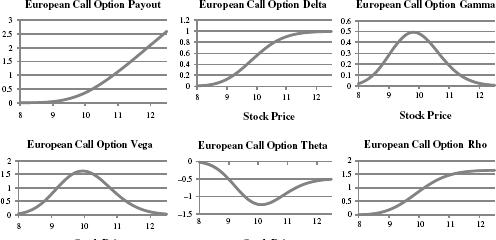
We can see, for example, that delta has an inflection point at $10 and that small movements around $10 result in the largest changes in delta as depicted by gamma. The delta on OTM calls rises at an increasing rate up to ATM and then at a decreasing rate. This should be clear from the sigmoid shape of delta and that is what gamma depicts, that is, that, while the option price is increasingly sensitive to the stock price up to $10, that sensitivity is somewhat muted once the option is in the money. Likewise, ATM option values have maximum sensitivity to changes in volatility (vega) but that sensitivity is muted somewhat away from $10. That is because as the spot price nears the strike, changes in volatility have bigger implications regarding whether the option will be in the money or not. Theta tells a similar, but inverted story; option value is most highly sensitive to the length of the contract (time to expiry) when the option is most out of the money. At the money, time sensitivity is lowest, and as an option moves further into the money, this sensitivity rises, but not as fast as it does as the option moves more and more out of the money. Like delta, rho rises monotonically with spot price, but at an increasing rate as the option approaches the strike price from below and at a decreasing rate as it moves further into the money. The intuition here is that small changes in the discount rate are more meaningful as the option approaches the strike price from any direction because near the money it has the greatest likelihood of making the option profitable (or not).
For puts, the boundary condition on Black-Scholes is c(S,T) = c(∞, t) = 0, and the solution to the Black-Scholes partial differential equation is:
![]()
The Greek letters for puts are the same as for those on call options. I also leave as an exercise the derivation of the option's rho; its sensitivity to interest rate changes. For a call, rho is equal to KTe^(–rT) N(d_2) and for a put, rho is –KTe^(–rT) N(–d_2).
![]() Go to the companion website for more details.
Go to the companion website for more details.
We can observe spot and exercise prices, discount rates, and time to maturity. But, as I argued in Chapter 11 on risk, we cannot observe volatility. This is the one input into option pricing models that must be estimated, either from historical data, or through revealed trades. Estimating volatility using observed option contracts is referred to as implied volatility. The VIX index is calculated as a weighted average of implied volatilities of various options on the S&P 500. We'll use the VIX in our risk hedging work in Chapter 18, on hedging risk. I set up an example in the Chapter 17 spreadsheet labeled Greeks using Excel's Solver and Black-Scholes that estimates volatility implied by an observed call option contract. This is a straightforward iterative exercise—given the market price of the option and conditional on the observed values for the discount rate, time to maturity, spot price, and strike price, we can back into the volatility implied by the observed price.
![]() Go to the companion website for more details (see Greeks under Chapter 17 examples).
Go to the companion website for more details (see Greeks under Chapter 17 examples).
Options traders often prefer to quote implied volatilities instead of prices. Consider, for example, the call option in Example 17.6 that trades at time t0 for $3.25 at spot price $36. The implied volatility is 20 percent. Suppose at time t1, the same five-month call is trading at $3.71, with the underlying price at $37. The implied volatility is now 15 percent. So, while the price of the call has increased, it has actually become cheaper in terms of volatility. What do we mean by cheaper in this context? The intuition has to do with the cost of hedging. Recall that for a delta hedge, we are long the stock and short the call and the stock hedges the risk that the call will be exercised. As the price of the stock rises, the cost of the hedge falls. Thus, in terms of implied volatility, this option is cheaper because it is cheaper to hedge.