Portfolio 3: Minimum Variance Portfolios with No Short Sales

Consider now the fully invested, minimum variance portfolio given by the solution to

but with the added (inequality) constraint that the weights must all be non-negative, that is,

This is an example of an inequality constraint; in this case, short sales are prohibited. The portfolio that solves this constrained minimization problem cannot be solved directly as we did for portfolios 1 and 2. Rather, we must iterate using numerical procedures (variants of Newton's method, for example). Excel has a data tool called Solver, which we can use to solve problems such as this. (Recall, we used Solver to find a solution to the linear programming problem of hedging future pension liabilities by selecting among several bonds of varying duration.)

To illustrate, let's take a look at a hypothetical three-asset portfolio with covariances and expected returns given by:

The diagonal of matrix A contains the asset return variances. The two off-diagonal elements indicate that asset 1 and asset 3 returns are positively correlated (, which you should verify) having covariance 0.2. I set this problem up purposely to show that without a no-shorting constraint, the optimizer will want to short asset 3. The intuition behind the short sale lies in the fact that asset 3 has both the highest risk and the lowest return, plus its risk is positively correlated with the risk on asset 1 (the lowest risk asset). Thus, it would be hard to make a case for taking a long position in asset 3 outside of a pure diversification argument (which, by the way is a powerful argument which you can see for yourself by experimenting with the covariances given in the spreadsheet to this chapter). The minimum-variance portfolio without a no-short sales restriction—that is, the solution using the method given in portfolio 1 is:

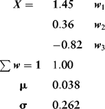
Notice the negative weight (–0.82) on asset 3 and the long weight (1.45) on asset 1, indicating that asset 1 has more than 100 percent weight; the sale of asset 3 was used to fund an increased allocation to asset 1. The expected return on this portfolio is 3.8 percent with volatility (risk) equal to 26.2 percent.

Let's now restrict short sales using Excel's Solver. Here is a snapshot of Solver's window with cell references from the chapter spreadsheet. Solver is asked to maximize the Sharpe ratio, μ/σ, by changing the weights (named wns for weights, no shorting) and restricting these weights to be non-negative. Thus, the Solver Parameters window looks like this:

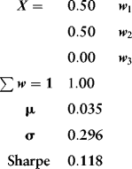
Solving gives the portfolio

Notice that the allocation to asset 3 binds on the constraint at zero. The expected return on any constrained portfolio will, by definition, be lower than that for unconstrained portfolios and that is borne out here as well (the return has fallen slightly to 3.5 percent). Risk must also be higher on the constrained portfolio (29.6 percent in this case). Intuitively, the absence of constraints allows the optimizer to search the entire weight space for the allocation that minimizes risk. Constraints restrict the available space for this search and therefore produce allocations that, while not globally optimal, are optimal in the restricted space.