Changing the Investment Horizon Returns Frequency

Investors have different investment horizons for a variety of reasons—liquidity needs and risk management, to name a few. I have included both weekly and daily closing prices for these 10 stocks and the S&P benchmark so that we could study the frequency implications to portfolio construction. Sticking with the five-year period ending in February 1997, I have constructed on wkly_r.xlsx in Chapter 7 Examples.xlsx, a time series of weekly returns. These are highlighted and their corresponding weekly means and standard deviations are given in rows 261 and 262. The covariance matrix is denoted by V_w and I have constructed two new portfolios that are the weekly analogs to the portfolios found on mthly_r.xlsx.

The first question that comes to mind is how changing the frequency alters the sample statistics like means and variances, and therefore the portfolio. If you compound the weekly mean returns in row 261, for example, to get monthly returns, and compare these to those found on mthly_r.xlsx, you will see that they are very close. (1 + rw)4 – 1 should be close to the monthly mean return rm. Or, if you prefer, multiply rw by 4 to get the arithmetic monthly equivalent. Likewise, σw√4 should be close to σm. The major point of interest, however, is in comparing optimal portfolios. I solve for both the minimum variance portfolio as well as a targeted return portfolio, in which the weekly targeted return compounds to the monthly targeted return of 3 percent solved for earlier. Table 7.2 shows the results.

Table 7.2 Changing the Returns Frequency.

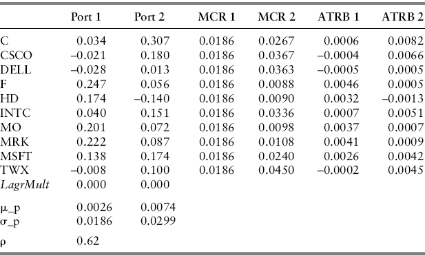
The mean return for Port 1, when compounded to monthly, is , which is slightly less than its monthly counterpart of 0.012. Comparing the risk to that on the minimum variance portfolio, we get 0.0186∗2 = 0.0372, which is slightly higher than the risk on the monthly counterpart. This is not supposed to be a big deal—we do not expect them to be the same—but it is important that they don't show wildly different results. More importantly, we ask how the allocation itself has changed. In this set of examples, there are significant differences. For example, the higher frequency weekly returns have a long position in C compared to the short position in the monthly frequency portfolio. Whereas the monthly portfolio is heavily tilted to Ford and Home Depot, the weekly portfolio also holds relatively heavy exposures to MO and MRK. Naturally, these differences will have implications concerning the marginal contributions to risk and to risk attribution in general. Why is this? Should observing market prices more frequently alter the risk-return trade-off that much? The short answer is yes and the reason is that higher frequency data contain more noise, which is embedded in covariance estimates. So, while the mean returns and risks seem to be fairly consistent across frequencies, their covariances may not be.

It is hard to compare covariances across frequencies; instead, we resort to comparisons of correlations, which are standardized covariances and, therefore, can be compared across any unit of measure. Recall that the correlation coefficient between two returns series rho:

Since we have 10 return series and covariances are symmetric, that is, , then we will have to estimate covariances (and correlations) plus N variances (and standard deviations). The covariance matrices V_m and V_w each have 45 covariances and 10 variances (the latter along the diagonal). If we divide each element in the covariance matrix by the product of the standard deviations of the two relevant returns series, then we can construct a correlation matrix. I did this for both the monthly and the weekly returns series. The Excel command is to highlight a area in the spreadsheet and then type the command:

Since σ_m is a row vector of standard deviations (I used STDEVP), then its transpose is a column vector and the product of an and a vector is an matrix, as you can see here:

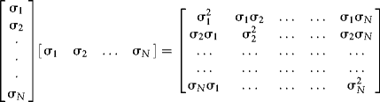
This is what we call an outer product (as opposed to an inner product, which consists of product sums). You should be able to see clearly that dividing the covariance matrix by this matrix produces exactly what we are after—a matrix of standardized covariances with ones along the diagonal.