Maximum Likelihood Estimation (Optional)

Although solving for MLE GARCH is beyond the scope of this book, it is instructive to see how MLE works for variance estimates in the homoscedastic case (single variance for all time). The intuition is that if we have a sample of returns r_i for i = 1,..., m, and that returns are independent and normally distributed, then the likelihood is the joint probability of seeing this particular sample. The parameters are then estimated to maximize this likelihood. For a sample of size m, the likelihood function can be written as the product of the individual likelihoods, since this is a joint likelihood (again, assuming the mean return to be zero)

Taking logarithms turns this product into a sum that is easier to work with and it does not affect the solution (note that we drop the constant , which has no impact on the solution).

To maximize this likelihood, take the derivative with respect to σ₂:

Solving this gets:

which is the familiar MLE of basic statistics courses. GARCH extends this logic to σ_i².

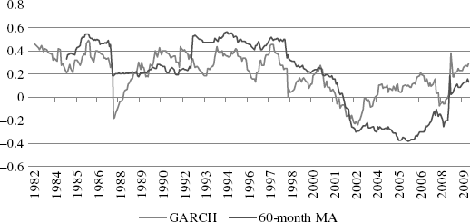
Multivariate GARCH models can estimate time-varying correlations and covariances. Figure 11.6 shows the correlation between fixed income and U.S. equity using a multivariate GARCH(1,1) setup. I used Matlab's UCSD toolbox and the dcc_mvgarch.m function.

Figure 11.6 Equity-Fixed Income Correlation

The time-varying nature of the correlation is obvious, but the points in which it turns negative may be a bit more subtle to some observers. Historical returns are provided on the spreadsheet labeled “Benchmark Correlations.” Notice, in particular, that during equity shocks such as the crash of October 1987, the bottom after the tech bubble crash, and the beginning of the credit crisis in early 2008 the correlations turn negative. During the “great moderation” of the latter part of the Greenspan Fed the correlation is rising (2001 to 2008), falls quickly below zero around the time that Bear Stearns failed and then spiked up again in the fall of 2008 when markets were locked into a systemic risk episode. It should be clear that the moving average correlation lags events considerably and in some cases misses them altogether.

The importance of changing volatilities and correlations should be obvious—portfolio optimization requires a covariance matrix. Up until now, we have been happy with a recursive covariance estimate using a sample of equal weighted returns history up to the present date. In this case, we are getting an average of the covariances. If, on the other hand, covariances and risk in general are regime-dependent, then standard recursive covariances are misspecified. That suggests that the optimized portfolio is as well. To see the intuition, consider again a two-asset portfolio of stocks and bonds. Using equal weighting, the covariance between these two asset classes is a historical average. If, however, we are in a phase in which the correlations have gone below zero but do not recognize that state, we are going to miss out on the diversification opportunities offered by negative covariances. Similarly, during periods in which correlations spike, standard covariance estimates will underestimate risk and overallocate as a result to the more risky assets. This is an excellent exercise to undertake as a test of your understanding on how covariance estimates affect asset allocation. Using the data in the spreadsheet to this chapter on fixed income (FI) and U.S. equity, use the MV GARCH correlations to construct a covariance matrix each month and, alongside the standard recursive covariance estimates, generate two optimal portfolios, rebalance each monthly, and compare their performance to a 70/30 benchmark of bonds and stocks.