Ito Processes

Ito processes are generalized Wiener processes in which the drift and volatility parameters can also be functions of S and t. That is:

Ito's lemma is a powerful result that allows us to find the price dynamic for a derivative of S. The intuition is that for any security, say, G, that we know to be a derivative of S, then Ito's lemma can be used to solve for the Brownian motion process of G. Ito's lemma says that G must satisfy the following relationship (A proof is given in Appendix 17.1):

---

Example 17.1

To illustrate, consider the following problem. Suppose a stock price follows a geometric Brownian motion, which is an Ito process . We want to find an expression describing the dynamics in the forward price F on a nondividend-paying stock, S with (T – t) time to delivery. That is, we want an expression for the security F given by the relationship if S follows an Ito process.

First, we recognize that the discount rate d(0,T) = e^–rT. We then compute the following partial derivatives according to Ito's lemma:

Making the necessary substitutions, we arrive at:

Finally,

This says that dF is also a geometric Brownian motion process with drift equal to the stock's risk premium.

---

---

Example 17.2 Proof of Lognormal Prices

Suppose governs the movements in the stock price S. What is the process governing movements in F = ln S(t)? To solve this, we use Ito's lemma. The process governing F is given by:

We next compute the partial derivatives:

Substituting these values into dF results in:

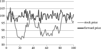
Figure 17.3 is one example of this returns process and its derivation is given in the chapter spreadsheet under the Generalized tab. Figure 17.4 shows the corresponding price dynamics for the forward contract from Example 17.1 and this stock. The example normalizes prices to start at 100 and assumes that the risk-free rate is 5 percent while the annualized return and volatility on the stock is 15 percent and 30 percent, respectively.

Figure 17.4 Application of Ito's Lemma

As Example 17.2 proves, there is less drift in the forward price. We can use this example to discuss confidence intervals and probability statements as well. Since the log price is normally distributed, we have in general:

Thus, if T corresponds to one year, say, and the stock return has mean μ equal to 7 percent with volatility-squared equal to 0.15² = 0.0225, then a 95 percent confidence band for simulated stock return will be contained in the range:

where –z = Normsinv(.025), z = Normsinv(.0975). Thus, the mean return is contained in the interval (−0.294, +0.294).

---