An Example

The basic building blocks for estimating the covariance matrix are return series for each of the underlying assets. In practice, analysts have several important decisions to make regarding the selection of these basic building blocks. Notably, they will want to choose historical data that are representative of the asset classes that they would consider including in their portfolios. For illustrative purposes, I have chosen common benchmarks for seven asset classes that are frequently considered by institutional investors. The qualitative results of this analysis were robust to the choice of alternative benchmarks for each of these asset classes, the inclusion of additional asset classes, using mixed frequency data, and return series with longer histories. Table 22.1 lists the return series that were chosen for each asset class and a risk-free rate, series inception date, and number of quarterly observations. Because the real estate and private equity return series are provided only quarterly, we geometrically linked the higher frequency returns to generate quarterly returns. All analysis in this paper was performed using quarterly excess returns, which were calculated by subtracting the risk-free rate from the aforementioned returns. Likewise, all results are presented in quarterly excess return format.

Table 22.1 Return Series Descriptions (All Data Ends December 2004)

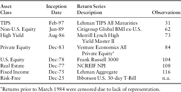
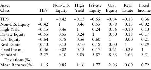
While all seven return series end in December 2004, their inception dates range from February 1997 for TIPS to December 1975 for fixed income. The differing inception dates normally force the truncation of longer time series in order to estimate covariances. A set of estimated correlations, standard deviations, and mean excess returns for the seven asset classes are presented in Table 22.2. Correlations are normalized covariances by dividing the latter through by the product of the two asset classes’ returns standard deviations. This means that variances (covariances between assets J and K where J = K) normalize to unity (diagonal elements in Table 22.2) while off-diagonal (J ≠ K) covariances normalize to correlations ρ, such that –1 ≤ ρ ≤ 1. These are the unconditional covariances based upon the truncated series. We will refer to these as the set of naïve estimates. Again, individual variances are estimated from each series’ history, while covariances are truncated to each common historical pairing.

Table 22.2 Naïve Correlation Matrix, Standard Deviations, and Mean Returns (Quarterly)

In the Monte Carlo study reported further on, we take the investment period to begin in the first quarter of 2005 and assume that all managers are mean-variance optimizers who estimate mean returns and covariances using information through 2004, solve the minimum variance portfolio, and hold that portfolio thereafter. We are especially interested in portfolio composition (that is, possible extreme positions), expected returns and risk.