Empirical Results

The naïve covariance estimates, which are equivalent to unconditional MLE for individual returns series but use the truncated series to estimate covariances are presented in Table 22.2. The set of corrected MLE returns, presented in Table 22.3, are the product of a two-step procedure in which we first remove the effects of smoothing from Private Equity and Real Estate returns by applying the Fisher-Geltner transformation outlined in Appendix 22.1. The covariance matrix was then estimated with a recursive application of Stambaugh's methodology in the following way:

Table 22.3 Corrected Correlation Matrix, Standard Deviations, and Mean Returns (Quarterly)

Return series were organized in descending order of length. The longest—fixed income, which dates to 1975—was used to estimate its own mean and variance. The next-longest series, real estate (unsmoothed), was then regressed against fixed income and the results were then used to update the conditional mean for real estate and its covariance with fixed income as given by equations (22.6) and (22.7). The returns to fixed income and real estate then constitute a matrix of instruments on which successively shorter returns series are regressed recursively, with covariances being revised according to equations (22.6) and (22.7). At the end of each recursion, the matrix of instruments is expanded once again. The new matrix of instruments is always truncated to a length equal to the series forming the next-longest series, the regression is estimated, and revisions made. That last regression involved TIPS, with a starting date of February 1997, and the matrix of instruments included the remaining six (unsmoothed) return series truncated to this date.

A comparison of Tables 22.2 and 22.3 22.3 indicate several sign reversals, most notably TIPS (the shortest series), and a scattered few for the remaining series. The results in Table 22.3 further suggest that TIPS is no longer so strongly and negatively correlated with U.S. equity, which highlights the informational differential between truncated and longer series. For example, variances and covariances based on short histories of truncated relationships will be overestimated if truncated series correspond to high volatility states. If short and long series are positively (negatively) correlated, then the conditional covariance MLE for the short series will be adjusted downward (upward) as indicated by equation (22.7). Its conditional mean, given by equation (22.6), will also be adjusted but the direction is uncertain; it will be adjusted downward when the truncated mean on the longer series exceeds its long-run average. This is an especially powerful result that shows how vulnerable covariance estimates are to shorter return series effects in the presence of truncation.

As discussed earlier, returns smoothing decreases volatility. The standard deviations increase significantly from Table 22.2 to Table 22.3 for private equity (5.87 percent to 9.13 percent) and real estate (1.66 percent to 4.36 percent). The naïve return volatility for TIPS, based on the truncated sample, is likewise revised upward from 2.27 percent to 3.38 percent. Other things constant, the naïve portfolio would have overallocated to these three asset classes and the magnitude of this misallocation rises with volatility underestimation.

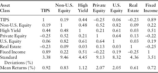
Figure 22.1 maps the efficient frontiers implied by each covariance matrix, using the naïve historical mean excess return for each asset class. These indicate quite clearly that the naïve covariance matrix underestimates risk and overestimates returns relative to the more efficient revised covariance matrix, a result consistent with Stambaugh's ((1997)) findings. The difference in the locations of the two frontiers is largely due to the underestimated standard deviations of the smoothed return series.

Figure 22.1 Efficient Frontier

A Monte Carlo Experiment

This section reports the results from a Monte Carlo study designed to answer the following question: Are both capital misallocation and portfolio performance significantly affected in the presence of substandard covariance estimates? Though we find that misallocation is indeed significant, and that portfolio performance suffers as a result, the magnitude and cost of misallocation will, in general, depend on the severity of truncation and smoothing and the number of affected assets. We present a simple case with two of seven assets having truncated returns and a third with smoothed returns.

The optimal portfolio corresponds to the vector of asset weights that solves the mean-variance optimization problem using as arguments a vector of mean returns and a covariance matrix. For the following experiment, we use as arguments the corrected parameter estimates given in Table 22.3, which consist of the unsmoothed Stambaugh-corrected covariance matrix and corresponding corrected mean returns. From these, we generate repeated samples of returns of length equal to 100 (25 years of quarterly returns) for each of the seven asset classes.

Specifically, if the estimated covariance matrix V is a positive definite, then it will have a Cholesky decomposition—a lower triangular square matrix A such that . Then, for any vector of mean returns μ, a single realization of a vector of simulated returns, with covariance structure given by V, can be generated from , where ε is a vector of standard normal random variables. Repeating this process over generates a sample of returns with mean and covariance , since is the identity matrix. For each generated sample, we truncate the simulated series for TIPS and non-U.S. equity to 25 and 50 periods, respectively, (these match the historical series lengths for TIPS and non-U.S. equity relative to fixed income), smooth real estate, and estimate covariances, and returns for three cases: (1) the full set of simulated returns—this is the portfolio based on full information, (2) the truncated and smoothed returns—our naïve model, and (3) the corrected means and covariances using Stambaugh and the Fisher-Geltner corrections. Separately, these sample mean-variance estimates were then used to solve the minimum variance, long-only, fully invested portfolio,

where V is case specific, that is, it corresponds to either the full information, naïve, or corrected covariance matrix.

Note that the choice of smoothing parameter, α, is 0.5 and was selected to generate a smoothed series that understates volatility by about one-half (empirically, we estimate this parameter in the range 0.4 – 0. Returns are smoothed according to , where is the smoothed return and r_t the actual return. The simulation program is available upon request.

The misallocation question was approached by measuring the sum of the absolute differences between the full-information weight vector in case (1) and the weight vectors in cases (2) and (3). This means we are interested in the distributions of the statistic:

where w^∗ denotes the full-information optimal portfolio, the optimal portfolio associated with either the naïve or corrected moments estimates, and N the number of replications in the experiment. We generate N matrices of returns each of size . Each matrix is then used to estimate expected returns and covariances for each of the three cases defined earlier, and these moment estimates solve three mean-variance efficient portfolios. Therefore, measures the absolute amount of misweighting between the full-information portfolio and each of the portfolios based on the naïve and corrected covariance estimates, respectively.

The weights in the preceding summation are matched pairs, by asset class, and their sum measures the aggregate deviation from the optimal portfolio weighting. The long-only constraint and absolute differences place an upper bound on the maximum misallocation equal to 2. Consider, for example, a two-asset problem. Maximum misallocation occurs when the two weight vectors are orthogonal, that is, w₁ = (0,1) and w₂ = (1,0) whose sum of absolute differences is equal to 2. Thus, the statistic , when divided by 2, measures the amount of misallocation, in percent, relative to the maximum allocation loss. Of primary interest is testing for relative misallocation, that is, whether is higher for the naïve model relative to the corrected covariance model. To this end, we drew samples of returns using the Monte Carlo method just described. A simple test of the null hypothesis that this statistic has zero mean is a parametric t-test on the coefficient in a regression of the difference in the paired returns on a constant. These t-statistics are supplemented with the nonparametric Wilcoxon test for matched pairs. Since z_n is a sum of absolute differences, its distribution is not necessarily normal; indeed, it is positive and skewed right. The nonparametric tests are distribution free and are reported as a check on the robustness of our results. Relevant statistics and test results are presented in Table 22.4. The Wilcoxon test is applied to the same three sets of matched pairs—the differences between the full-information portfolio and each suboptimal portfolio (that is, the naïve and corrected portfolios) and a third, measuring the difference between the naïve and corrected portfolios. Wilcoxon is a test of medians; specifically, that the median of the differenced distribution (the paired differences) is zero, that is, the two returns distributions share a common central tendency.

Table 22.4 Monte Carlo Simulation Results.

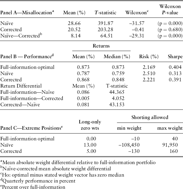
Panel A of Table 22.4 shows that the average misallocation for the naïve portfolio is 28.66 percent and the test of Wilcoxon easily rejects the null that they share a common median. Using the Stambaugh and Fisher-Geltner corrections reduces misallocation to 20.52 percent, which is about 8.14 percent less, but interestingly, the test of Wilcoxon cannot reject the null that the corrected and full-information weight distributions share the same median. Clearly, though, the mean misallocation difference between the naïve and corrected covariance portfolios is significant and, in this case, about 8.14 percent on average in each quarter.

Portfolio performance measures are straightforward computations using expected returns, which are the product of the mean-variance optimal weights and mean returns specific to each case , and portfolio risk , where again, w is the case specific mean-variance optimal weight vector and V is the case-specific estimated covariance matrix. Results, which are presented in Panel B of Table 22.4 show that misallocation results in more extreme positions as evidenced by lower portfolio returns and higher portfolio risk. Indeed, the median quarterly return under the naïve approach (0.787 percent) underperforms both the optimal return (0.873 percent) by 0.086 percent per quarter and the corrected covariance case (0.896 percent) by a little over 0.081 percent per quarter. The naïve portfolio's tendency to take extreme positions can be seen in the volatility of its returns; 2.51 percent per quarter relative to 2.16 percent and 2.22 percent for the full information and corrected cases, respectively, as well as the lowest Sharpe ratio (measured over the 10,000 replications).

The long-only constraint places bounds on extreme positions. Nevertheless, Panel C reports that naïve portfolios contain approximately 13 percent more extreme positions v(zero positions on an asset class) while portfolios generated from the corrected moment estimates produce roughly 5 percent more zero positions relative to the optimal portfolio. When the long-only constraint is removed, extreme positions are accentuated but only for the naïve case. Here, the range of weights for the naïve case is huge (–108,450 percent to 91,950 percent) while those for the corrected covariance case (–130 percent to 160 percent) and the optimal full-information case (–10 percent to 40 percent) remain reasonably narrow. The weight range for the naïve case is not due to outliers; indeed, the interquartile range is about 300.

The naïve model's rather significant tendency to bias portfolio weightings generates increased risk primarily because it misallocates capital to the wrong asset classes. Bias, itself, tends to favor the smoothed series and, to the extent that a truncated series is currently experiencing a period of low volatility, bias overweights those assets as well. As a result, the naïve model will produce understated value-at-risk estimates, which may lead managers to take on bets that are not otherwise supported by the data. The magnitude of the weighting bias is a function of both the proportion of assets with limited histories and their relative series lengths—shorter histories will exacerbate the bias, as will the magnitude of smoothing.