Overlapping Observations

A final topic concerns the analysis of returns series constructed on moving windows of historical returns. It is common, for example, to smooth the noise in observed returns by constructing moving averages. An example is Shiller's 10-year moving average of trailing earnings on the S&P 500 that he uses to filter noise in earnings. This smoothed earnings number is used to estimate the p/e ratio. Three-year or five-year moving averages of monthly returns or volatilities, for example, are often found in presentations of portfolio performance. A three-year moving average will typically construct the current month smoothed return, using a sample of 36 months of trailing returns. A time series of three-year moving averages means that adjacent months have 35 observations in common. Observations on the moving average that are two months removed have 34 observations in common and so on. Since the moving averages overlap in this fashion, they constitute a serially correlated time series, and this property has implications concerning the information content of the newly constructed series as well as its statistical properties.

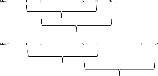
Let's think about the information content first. The reason the assumption of independence of returns is so attractive is that each return can be thought of as a truly novel byte of information. Independence implies that there are N distinct bytes of information in a sample of size N. So, for example, if returns were independently distributed across time, then a three-year trailing sample of monthly returns contains 36 independent sources of information. Serially correlated observations, by construction, remove that property. Two adjacent moving averages constructed off of 36-month trailing returns hardly constitute independent sources of information simply because they contain so much in common. Moreover, the dependence of the moving averages is embedded for some time to come. For example, we require the passage of 36 months to remove this dependence. Figure 22.2 illustrates this property. The top panel shows the obvious dependence of overlapping returns at the one-month interval while the bottom panel shows how slow this dependence deteriorates.

Figure 22.2 Serial Dependence of Moving Averages of 36-Month Trailing Returns

This dependence structure seriously limits the information content of time series constructed on moving averages. A three-year time series of 36-month moving averages, for example, has only a single truly independent observation because technically all of the observations in this sample are correlated. This behavior poses certain challenges to how we approach the measurement of various statistics, the most important one being volatility estimates. You may recall from basis statistics that the standard deviation of a sample of returns is based on the assumption that the returns are independently distributed. If they are serially correlated instead, then one has to make corrections to adjust for that property. The case most students are familiar with addresses correcting for serial correlation in the estimator of the residual variance from a linear regression. A model of first order serial correlation, for example, can be written as follows:

Here, –1< ρ < 1 is the correlation coefficient and (identically and independently distributed random variables) and the ε_t are the residuals. If we compute the variance of ε, we get:

This says that the true variance is understated by a factor of . So, if ρ = .9, then the true variance is understated by 10. The parameter ρ is telling us how much information is common (and therefore not unique) to adjacent observations. Smoothing (as in moving averages) creates serial correlation and the observed variance of moving averages created by overlapping data will therefore filter the underlying volatility. We adjust for this smoothing by dividing by (1 – ρ²).

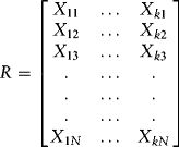
Let's make an attempt to generalize this concept. Suppose we have a time series of N demeaned returns on K stocks, each denoted by X_ij as follows:

The covariance matrix we studied in previous chapters was estimated by (assuming returns are demeaned already), . That estimator assumed that returns were independent and identically distributed (IID). Let us now allow for serial correlation of order m; for example, each of these returns could be an mth-order moving average. An estimator for V that is a positive definite (V has full rank and is invertible) is given by Newey-West (1987) and can be written for our case here as follows:

This is a sum of (positive semi-definite) covariance matrices. V₀ is the covariance estimated from the smoothed data with no adjustment for serial correlation. The adjustment factors are covariance matrices that estimate the serially correlated covariances. Assuming X = R is a matrix of demeaned returns, then is a covariance estimate for X and its jth lag. For example, let's consider the case in which X_ij could be a three-month moving average of returns so that m = 2. The March moving average is the average of January, February, and March. The April moving average is the average of February, March, and April. Hence, they have m = 2 months overlap. Then is correlated with as well as and this is why –m ≤ j ≤ m. The chapter spreadsheet labeled Overlapping has a sample of demeaned monthly returns for Citigroup and Cisco spanning April 1992 to December 2006. Columns B and C contain the demeaned returns and columns D and E contain three-month moving averages of these returns. The unadjusted covariance matrix is given at the top of the sheet:

The Newey-West adjusted covariance is given at the top of columns R and S as:

Clearly, no adjusting for serial correlation would have led to a significant underestimate in the risk matrix. Fortunately, Newey-West estimators are available in most software packages so one can avoid having to construct these adjustments individually.