Discounting Using Spot Rates

There are plenty of excellent treatments of the term structure. I therefore keep this chapter short and to the point. The yield curve is a plot of Treasury spot rates. The spot rate is the current market interest rate for a given term (for example, the yield on the one-year Treasury bill). For example, lending $1 at 10 percent for a single year means that the one-year spot rate is 0.10. If you were to lend the $1 for a period of two years at 10 percent annually, then the two-year spot rate is also 0.10. So, for the one-year spot, s₁, and a $1 investment, the factor by which that investment will grow is . For the same $1, over two years, that investment will grow to , or 100^∗s₂ percent in each of two years. In general, then, $1 will grow at for a period of t years at an annual rate equal to s_t. If the rate is compounded m times per year, then this changes to: . And, if the rate is compounded continuously, then as we have shown before, , where the second time term (t) denotes the span of years. Discounting is just the inverse operation. For example, a cash flow of $1 that is to be realized in t years has value at the present time. If interest is compounded m times per year, then the discount factor d(t) becomes , and if continuously compounded, . 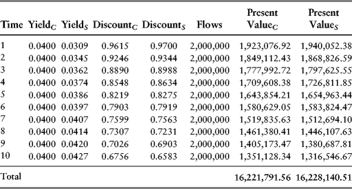Moreover, if we knew the term structure of spot rates, then a cash flow stream through time of to be received in periods has present value , where the d_i are the aforementioned discount factors. Notice that this formulation is different from that for valuing bond-paying coupons . The difference is that in the bond valuation case, we determined the internal rate of return (the yield to maturity), which was a single discount factor; it was a geometric mean (see Chapter 1). In reality, if one knew the spot rates for differing time periods, then one could discount a stream of cash flows using the proper discount factors and not a single factor like the yield to maturity. Keep in mind, however, that the purpose of calculating yield to maturity on a bond was to find a unique rate of return that equated the present value of a cash flow stream to its market price.

---

Example 3.1

As an example, suppose the interest rate is constant at 4 percent, implying that the yield curve is flat. When applied to a 10-year stream of net cash flows, each of which is $2 million, the estimated present value is for t = 1,...,10. The discount factors d(t) are here. This method would certainly give misleading results if the yield curve were not flat. The point here is that we always seek the proper discount factor; rarely is it constant over time, and any example that assumes so is going to produce some model error as a result. That's why you should recompute this PV using the proper set of discount rates. Suppose the proper set of discount rates (Disc_S) were based on the following term structure of interest rates (Yield_S) (from Chapter 3 Examples.xlsx).

Table 3.1 Fixed versus Floating Discount Factors

Thus, while the PV was $16,221,791.56 using a constant 4 percent discount rate, it is now $16,228,140.51. In general, we would prefer to use discount rates that more precisely match the market's time preferences, which would suggest working with the term structure of interest rates and their implied forward rates.

Go to the companion website for more details.

---