
Duration Redux
In the previous chapter, we worked exclusively with a flat term structure, in which interest centered on the sensitivity of bond prices to a change in yield, ![]() . The assumption of a flat term structure is very restrictive. What happens when we relax this constraint? In a world in which spot rates differ across maturities, interest rate risk and duration are no longer tied to a single yield but to the entire term structure; more specifically, to movements in the term structure. That is, we now wish to evaluate
. The assumption of a flat term structure is very restrictive. What happens when we relax this constraint? In a world in which spot rates differ across maturities, interest rate risk and duration are no longer tied to a single yield but to the entire term structure; more specifically, to movements in the term structure. That is, we now wish to evaluate ![]() , where the
, where the ![]() are the spot rates that vary across maturities and Δ is a constant that shifts the term structure up or down in a parallel fashion. Parallel shifts are also restrictive but a necessary simplification—since we cannot control for spot rates varying independently by random amounts we instead study parallel shifts
are the spot rates that vary across maturities and Δ is a constant that shifts the term structure up or down in a parallel fashion. Parallel shifts are also restrictive but a necessary simplification—since we cannot control for spot rates varying independently by random amounts we instead study parallel shifts ![]() .
.
With continuous compounding, the bond price formula from the previous chapter becomes:
![]()
If the cash flows are constant across time, then ![]() . As before, duration is the weighted sum of the elapsed times to wait for cash flows divided by the bond price, that is,
. As before, duration is the weighted sum of the elapsed times to wait for cash flows divided by the bond price, that is,
![]()
We call this the Fisher-Weil duration. If we shift the term structure by Δ, then the price of the asset changes accordingly:
![]()
We seek the delta of the asset given by the derivative evaluated at Δ = 0:
![]()
This is not only convenient, it is also essentially the primary result we derived in the previous chapter, ![]() .
.
Let's expand our thinking to pricing general cash flow streams that include everything from bonds to mortgages to installment loans. Since many of these loans pay interest periodically, then their valuations will be sensitive to changes in rates as well as their periodicity (compounding). As an example, consider a typical installment loan that makes payments m times per year. We therefore have the familiar pricing model given by:
![]()
Interest rate risk is therefore:
![]()
We can derive the quasi-modified duration measure by dividing both sides by P:
![]()
This is rather cumbersome but not difficult to code onto a spreadsheet, as we can see in Example 3.5.
Example 3.5 Table
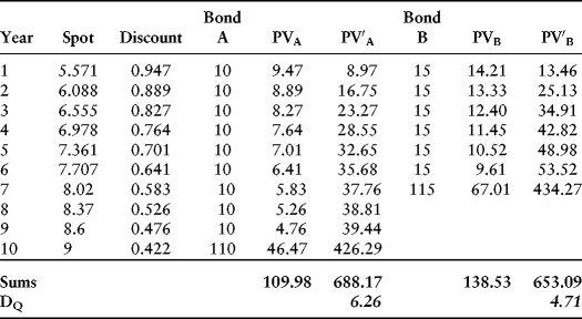
The quasi-modified duration is given in the last row: 6.26 years and 4.71 years for bonds A and B, respectively. Our obligation has present value equal to $1M ∗ 0.701 = $701,079.49. As before, we want a portfolio of the two bonds such that the present value of the portfolio's cash flows is equal to the present value of the liability. Also, the sum of the duration-weighted present values will equal the duration-weighted present value of the liability. Once again, therefore, we require the two conditions:
![]()
![]()
Setting up the algebra, we wish to solve the following system of two equations:
![]()
We can solve this by elimination as we did in Chapter 2 or by using matrix algebra, which I illustrate here because it is so much more practical, especially for larger problems involving more unknowns. First, write the problem algebraically in matrix form as follows:
![]()
Call this system Ax = b, where A is 4 × 4 and x and b are the two 2 × 1 column vectors. (The appendix to Chapter 6 contains a review of matrix algebra). We want the solution x = A–1b which, consulting the worksheet examples for this chapter (Example 3.5) yields ![]() . The value of this portfolio is exactly $701,079.49. Note that bond B is overweighted because its duration is close to the duration of the liability.
. The value of this portfolio is exactly $701,079.49. Note that bond B is overweighted because its duration is close to the duration of the liability.
What happens if there is a parallel shift in the yield curve? Column K on the worksheet represents a 1 percent upward shift in the yield curve. Copying and pasting this vector over the old spot rates in column B (copy/paste special/values) indicates that the present value of the obligation is now equal to $669,321.81, which is exactly offset by the value of the portfolio which, again, contains a short position in bond A. Note as well that the duration on both bonds have declined because of the heavier discounting associated with the higher yield curve.