The Efficient Frontier (Again)
![]() Go to the companion website for more details (see Efficient Frontier under Chapter 06 Examples).
Go to the companion website for more details (see Efficient Frontier under Chapter 06 Examples).
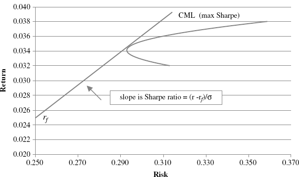
We can use the two-fund theorem to construct our efficient frontier (see Figure 6.1). Recall that this theorem states that the set of efficient funds (portfolios) can be constructed as linear combinations of any two efficient portfolios. We have two minimum variance and, hence, efficient portfolios from portfolios 1 and 2. I form a bunch of new funds as linear combinations of these two funds on the Efficient Frontier sheet in Chapter 6 Examples.xlsx. To do this, I need the return and risks for the two portfolios and their correlation coefficient ρ. I also need a set of weights that I use to form linear combinations of these two portfolios. The only restriction is that the two weights must sum to one. The gradation of the weights is not important, but you can see from the spreadsheet that I generated enough to get a smooth graph of the frontier. Here it is:
Figure 6.1 Efficient Frontier

I assume the risk-free rate is 2.5 percent. The line tangent to the efficient set is the capital market line. We already showed that it has slope ![]() and intercept equal to the risk free rate rf. It has maximum slope at the point of tangency with the efficient set—this is portfolio 5, with a risk-free rate of 2.5 percent; it is the portfolio with the maximum Sharpe ratio. If we refer to the Efficient Frontier spreadsheet, we see that the tangency portfolio consists of equal parts of Portfolios 1 and 2 that we derived earlier. This is an important result. It means that all we need own is this portfolio (the tangency portfolio) and lend or borrow at the risk-free rate to maximize utility. Everyone, regardless of the form of her utility functions, can do likewise.
and intercept equal to the risk free rate rf. It has maximum slope at the point of tangency with the efficient set—this is portfolio 5, with a risk-free rate of 2.5 percent; it is the portfolio with the maximum Sharpe ratio. If we refer to the Efficient Frontier spreadsheet, we see that the tangency portfolio consists of equal parts of Portfolios 1 and 2 that we derived earlier. This is an important result. It means that all we need own is this portfolio (the tangency portfolio) and lend or borrow at the risk-free rate to maximize utility. Everyone, regardless of the form of her utility functions, can do likewise.
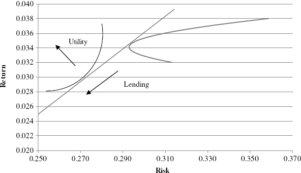
Figure 6.2 illustrates this concept. The CML contains the tangency portfolio and includes a set of points all of which are preferred to any other point on the efficient frontier. That is, all points on the CML have higher return and risk. If we express peoples’ utility functions in risk and return space—I impose a representative indifference curve that is tangent to the CML to illustrate—then we can see that, depending on individual risk appetites, the utility-maximizing investor can choose to hold the tangency portfolio (the market), lend by holding a mix of the market portfolio and the risk-free asset (as shown in Figure 6.2), or borrow by shorting the risk-free asset in order to achieve higher expected returns and risk by moving to the northeast along the CML.
Figure 6.2 Maximizing Utility by Borrowing or Lending

