Performance Attribution

The following summarizes some relevant parameter values and performance statistics.

Table 10.1 Performance Summary and Parameter Values.

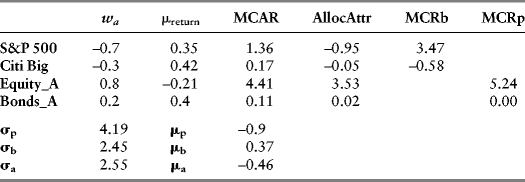
The first column obviously shows the short position in the benchmark and the equity tilt in the active portfolio. The second column shows the average monthly returns to the benchmark and active portfolios during the evaluation period. Note the negative return to the active equity portfolio. The third column contains the marginal contributions to active risk (MCAR). These tell us how active risk changes on the margin for a 1 percent increase in the allocation to the portfolio in question. The active risk σ_a is equal to 2.55 percent (monthly). The allocation to equity in the active portfolio is 0.8. Since MCAR is a derivative, , it returns the change in active risk (from 2.55 percent) for a one-unit change in the active weight (0.8 to 1.8). We need to rescale this weight change for it to make sense. Thus, a change from 0.8 to 0.9 (dw_a = 0.10, in this case) implies a change in active risk of 0.441, which bumps σ_a to 2.99 percent.

This is a powerful feature of risk management. It tells us how our portfolio risk changes along the margins. Obviously, active risk is much more sensitive to small changes in the allocation to the active equity portfolio; for example, an equivalent allocation increase to active bonds (from 0.2 to 0.3) would raise active risk from 2.55 percent to about 2.56 percent. This shows us just how much riskier the equity manager is relative to the bond manager. That's a lot of risk for 50 bps of annualized return over the benchmark!

The allocation attribution (AllocAttr) simply parses risk across the portfolio. Summing the elements in this column give us 2.55 percent. Obviously, the active equity portfolio accounts for more than 100 percent of this (3.53 percent) but is offset somewhat by the short position in the benchmark (–0.95 percent).

The last two columns are there to illustrate that marginal contributions to risk are not confined to the active portfolio; we can compute these derivatives for the benchmarks and the active portfolios separately as:

Notice that w_a is 2 × 1, showing the deviations in the active portfolio from the long-run benchmark. This measure informs us of the cost of deviating from the benchmark. Similarly, we can compute marginal risk directly on the active portfolio:

Each measure is a gradient-measuring slope along the risk surface. Chapter 11 develops these concepts in greater detail. For the moment, recognize that there are measures of total risk (for example, σ_a = 2.55 percent), which is a static concept, as well as risk sensitivity along the margins, which gives a clear picture on what our risk function looks like in the neighborhood of the current allocation.

One big question remains—how good did the active managers do? Clearly, there's a lot of unwelcome risk carried in the active equity portfolio, but did it pay off? The simple answer is no. We see that the mean return to the active portfolio (0.8^∗Equity_A + 0.2^∗Bonds_A) is negative at –0.9 per month while the benchmark portfolio (0.7^∗S&P 500 + 0.3^∗Citi BIG) is 0.37 per month. The difference between them is –0.46 per month, which translates into about –0.46^∗12, or –5.52 percent per year under performance. That's because of the aggressive equity style. In fact, if we were to regress RpA on Rb, we'd get the following result:

The t-statistics are –2.03 and 11.45, respectively, indicating that they are both statistically significant. Thus, the trustees did not get the alpha they anticipated. Rather, the active portfolio underperformed by 0.62 percent per month while the beta estimate of 1.43 says that the active portfolio had 43 percent more risk than the benchmark portfolio. This means that the active managers were not contributing skill per se, but were simply taking more equity risk relative to the benchmark. Using the mean benchmark return of 0.37 percent per month, I estimate that the expected annual return attributable to this active strategy would have been –1.09 percent.

This is admittedly a contrived example, but it is instructive nevertheless. The mean-variance efficient portfolios are given on the “Active Positions” tab. You can see here that the equity portfolios are heavily tilted toward HD, MO, and MRK and F, of which only MO had a positive average return over the evaluation period. The two remaining firms with average positive returns, C and CSCO, by contrast, had much smaller allocations. The covariance estimates were steering the optimizer toward these exposures in 10 firms that had essentially little to offer in the way of return. That and the aggressive strategy forced a highly risky allocation that could not outperform the benchmark, which, itself, had a comparatively good track record. For the bond fund, performance was somewhat more muted, but clearly, the allocation was almost entirely COLL (not surprising since the risks are so much closer together for these bonds sectors compared to the 10 equities). The active bond portfolio missed out on the relatively better return record offered by CRED over the evaluation period. Nevertheless, let's not read into these results too much. The purpose of the exercise was to demonstrate performance attribution methodologies and not portfolio selection.