11

One-Way ANOVA with One Repeated-Measures Factor

Overview

This chapter shows how to perform one-way repeated-measures ANOVA using the Fit Model platform in JMP. The focus is on repeated-measures designs, in which each participant is exposed to every condition under the independent variable. This chapter describes the necessary conditions for performing a valid repeated-measures ANOVA, discusses alternative analyses to use when the validity conditions are not met, and reviews strategies for minimizing sequence effects.

Overview

Introduction: What Is a Repeated-Measures Design?

Example with Significant Differences in Investment Size across Time

Designing the Study

A Univariate Approach for Repeated Measures Analysis Using the Fit Y by X Platform

Summarize the Results of the Analysis

Formal Description of Results for a Paper

Repeated-Measures Design versus the Between-Subjects Design

Weaknesses of the One-Way Repeated Measures Design

Sequence Effects

Univariate or Multivariate ANOVA for Repeated-Measures Analysis?

Review the Data Table for a Multivariate Analysis

Using the Fit Model Platform for Repeated-Measures Analysis

Steps to Review the Results

Summarize the Results of the Analysis

Formal Description of Results for a Paper

Summary

Appendix: Assumptions of the Multivariate Analysis of Design with One Repeated-Measures Factor

References

Introduction: What Is a Repeated-Measures Design?

A one-way repeated-measures ANOVA is appropriate when

• the analysis involves a single nominal predictor variable (independent factor) and a single numeric continuous response variable (dependent variable)
• each participant is exposed to each condition under the independent variable

The repeated-measures design derives its name from the fact that each participant provides repeated scores on the response variable. That is, each participant is exposed to every treatment condition under the study’s independent variable and contributes a response score for each of these conditions. Perhaps the easiest way to understand the repeated-measures design is to contrast it with the between-subjects design, in which each participant participates in only one treatment condition.

For example, Chapter 8, “One-Way ANOVA with One Between-Subjects Factor,” presents a simple experiment that uses a between-subjects design. In that fictitious study, participants were randomly assigned to one of three experimental conditions. In each condition, they read descriptions of a number of romantic partners and rated their likely commitment to each partner. The purpose of that study was to determine whether the level of rewards associated with a given partner affected the participant’s rated commitment to that partner. The level of rewards was manipulated by varying the description of one specific partner (partner 10) that was presented to the three groups. Level of rewards was manipulated in this way:

• participants in the low-reward condition read that partner 10 provides few rewards in the relationship
• participants in the mixed-reward condition read that partner 10 provides mixed rewards in the relationship
• participants in the high-reward condition read that partner 10 provides many rewards in the relationship

After reading one of these descriptions, each participant rated how committed he or she would probably be to partner 10.

This study is called a between-subjects study because the participants were divided into different treatment groups (reward groups) and the independent variable was manipulated between these groups. In a between-subjects design, each participant is exposed to only one level of the independent variable. In this case, a given participant read either the low-reward description, the mixed-reward description, or the high-reward description. No participant read more than one description of partner 10.

On the other hand, each participant in a repeated-measures design is exposed to every level of the independent variable and provides scores on the dependent variable under each of these levels. For example, you could modify the preceding study so that it becomes a one-factor repeated-measures design. Imagine that you conduct a study with a single group of 20 participants instead of three treatment groups. You ask each participant to go through a stack of potential romantic partners and give a commitment rating to each partner. Imagine further that all three versions of partner 10 appear somewhere in this stack, and that a given participant responds to each of these versions.

For example, a given participant might find the third potential partner to be the low-reward version of partner 10 (assume that you renamed this fictitious partner to be “partner 3”). This participant gives a commitment rating to partner 3 and moves on to the next partner. Later, the 11th partner happens to be the mixed-reward version of original partner 10 (now renamed “partner 11”). The participant rates partner 11. Finally, the 19th participant happens to be the high-reward version of partner 10 (now renamed “partner 19”). The participant rates partner 10 and finishes the questionnaire.

This study is now a repeated-measures design because each participant is exposed to all three levels of the independent variable. One way to analyze the data is to create one variable for each of the commitment ratings made under the three different conditions:

• One variable (call it low) contains the commitment ratings for the low-reward version of the fictitious partner.
• One variable (mixed) contains the commitment ratings for the mixed-reward version of the fictitious partner.
• One variable (high) contains the commitment ratings for the high-reward version of the fictitious partner.

To analyze repeated-measures data in this form, you compare the mean scores for these three variables. Perhaps you hypothesize that the commitment score for high is significantly higher than the commitment scores for low or mixed.

Make note of the following two cautions before moving on.

• Remember that you need a special type of statistical procedure to analyze data from a repeated-measures study. You should not analyze the data using the Fit Y by X platform to do a one-way ANOVA, as illustrated in Chapter 9.
• The fictitious study described here was used to illustrate the nature of a repeated-measures research design—do not view it as an example of a good repeated-measures research design. In fact, the preceding study suffers from several serious problems. Repeated-measures studies are vulnerable to problems not encountered with between-subjects designs. Some of the problems associated with this design are discussed later in the “Sequence Effects” section.

Example with Significant Differences in Investment Size across Time

To demonstrate the use of the repeated measures ANOVA, this chapter presents a new fictitious experiment that examines a different aspect of the investment model (Rusbult, 1980). Recall from earlier chapters that the investment model is a theory of interpersonal attraction. The study describes variables that determine commitment to romantic relationships and other interpersonal associations.

Designing the Study

Some of the earlier chapters described investigations of the investment model that involved the use of fictitious partners. They included written descriptions of potential romantic partners to which the participants responded as if they were real people. Assume that critics of the previous studies are very skeptical about the use of this analogue methodology and contend that investigations using fictitious partners do not generalize to how individuals actually behave in the real world. To address these criticisms, this chapter presents a different study that could be used to evaluate aspects of the investment model using actual couples.

This study focuses on the investment size construct from the investment model. Investment size refers to the amount of time, effort, and personal resources that an individual puts into a relationship with a romantic partner. People report heavy investments in a relationship when they have spent a good deal of time with their romantic partner, when they have a lot of shared activities or friends that they would lose if the relationship were to end, and so forth.

Assume that it is desirable for couples to believe they have invested time and effort in their relationships. Further, this perception is desirable because research has shown that couples are more likely to stay together when they feel they have invested more in their relationships.

The Marriage Encounter Intervention

Given that high levels of perceived investment size are a good thing, assume that you are interested in finding interventions that are likely to increase perceived investments in a marriage. Specifically, you read research indicating that a program called the marriage encounter is likely to increase perceived investments. In a marriage encounter program, couples spend a weekend together under the guidance of counselors, sharing their feelings, learning to communicate, and engaging in exercises intended to strengthen their relationship.

Based on what you have read, you hypothesize that couples’ perceived investment in their relationships increases immediately after participation in a marriage encounter program. In other words, you hypothesize that, if couples are asked to rate how much they have invested in a relationship both before and immediately after the marriage encounter weekend, the post (after) ratings will be significantly higher than the pre (before) ratings. This is the primary hypothesis for your study.

However, being something of a skeptic, assume further that you do not expect these increased investment perceptions to endure. Specifically, you believe that if couples rate their perceived investment at a follow-up point three weeks after the marriage encounter weekend, these ratings will have declined to their initial pre-level ratings, which were observed just before the weekend. In other words, you hypothesize that there will not be a significant difference between investment ratings obtained before the weekend and those obtained three weeks after the weekend. This is the secondary hypothesis for your study.

To test these hypotheses, you conduct a study that uses a single-group experimental design with repeated measures.

Figure 11.1: Single-Group Experimental Design with Repeated Measures

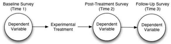
Suppose you recruit twenty couples who are about to go through a marriage encounter program. The response variable in this study is perceived investment measured with a multiple-item questionnaire. Higher scores on the scale reflect higher levels of perceived investment.

Each couple gives investment ratings at the three points in time illustrated by the three circles in Figure 11.1. Each circle represents one dependent variable. Specifically,

• a baseline survey obtains investment scores at Time 1, just before the marriage encounter weekend
• a post-treatment survey obtains investment scores at Time 2, immediately after the marriage encounter weekend
• a follow-up survey obtains investment scores at Time 3, three weeks after the marriage encounter weekend

Notice that an experimental treatment, the marriage encounter program, appears between Time 1 and Time 2.

Problems with Single-Group Studies

Keep in mind that the study described here uses a weak research design. To understand why, remember the main hypothesis you want to test is that investment scores increase significantly from Time 1 to Time 2 because of the marriage encounter program. Imagine for a moment that the results obtained when you analyze the study data show that Time 2 investment scores are significantly higher than Time 1 scores.

These results do not provide strong evidence that the marriage encounter manipulation caused the increase in investment scores. There are obvious alternative explanations for the increase. For example, perhaps investment scores naturally increase over time among married couples regardless of whether they participate in a marriage encounter weekend. Perhaps an increase in score is due to simply having a restful weekend and not due to the marriage encounter program at all. There is a long list of possible alternative explanations.

The point is that you must carefully design repeated-measures studies to avoid confounding the response and other problems. This study is for illustration only, and is not designed very carefully. The “Sequence Effects” section later in this chapter discusses some of the problems associated with repeated-measures studies and reviews strategies for dealing with them. In addition, Chapter 12, “Factorial ANOVA with Repeated-Measures Factors and Between-Subjects Factors,” shows how you can make the present single-group design stronger by including a control group.

Predicted Results

The primary hypothesis is that the couples’ ratings of investment in their relationships increases immediately following the marriage encounter weekend. The secondary hypothesis is that this increase is a transient or temporary effect rather than a permanent change. These hypothesized results appear graphically in Figure 11.2. Notice that mean investment scores increase from Time 1 to Time 2, and then decrease again at Time 3.

Figure 11.2: Hypothesized Results for the Investment Model Study

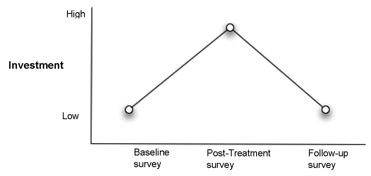
You test the primary hypothesis by comparing post-treatment (Time 2) investment scores to the baseline scores (Time 1). Comparing the follow-up scores (Time 3) to the baseline scores (Time 1) shows whether any changes observed at post-treatment are maintained and use this comparison to test the secondary hypothesis.

Assume this study is exploratory because studies of this type have not previously been undertaken. Therefore, you are uncertain what methodological problems might be encountered or the magnitude of possible changes. This example could serve as a pilot study to assist in the design of a more definitive study and the determination of an appropriate sample size. Chapter 12, “Factorial ANOVA with Repeated-Measures Factors and Between Subjects Factors,” presents a follow-up study based on the pilot data from this project.

A Univariate Approach for Repeated Measures Analysis Using the Fit Y by X Platform

Twenty couples participated in this study. Suppose that only the investment ratings made by the wife in each couple are analyzed. The sample consists of data from the 20 married women who participated in the marriage encounter program.

The response variable in this study is the size of the investment the participants (the wives) believe they have made in their relationships. Investment size is measured by a scale that gives a continuous numeric value.

Review the JMP Data Table

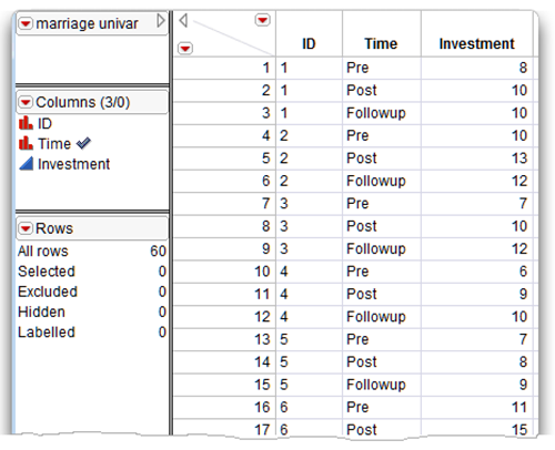
The JMP data table called Marriage univar.jmp lists the investment scores obtained at the three different points in time for 20 participating couples. Each couple (each wife) contributes three rows to the data table.

• The nominal variable, ID, identifies each couple with values “1” through “20.” Each couple contributes three lines of data corresponding to the three time periods.
• The nominal variable, time, identifies the time period with values “Pre,” “Post,” and “Followup.”
• The continuous numeric investment score variable, investment, lists the investment scores recorded at each time period.

Figure 11.3 shows a partial listing of the 60 observations in the data table.

Figure 11.3: Partial Listing of the marriage univar Data Table

Plot the Mean Investment Scores

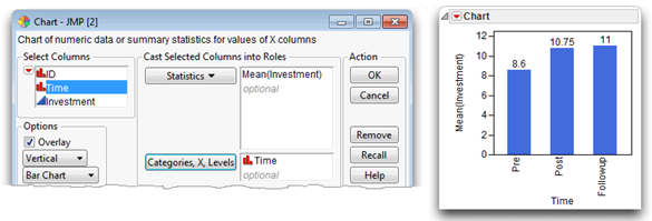
You can quickly compare the mean investment scores for each time period by using the Chart platform, as follows:

Choose Chart from the Graph menu.

On the Chart launch dialog, select Time in the Select Columns list, and click X, Level.

Select Investment in the Select Columns list, and choose Mean from the Statistics menu in the dialog.

Click OK to see a bar chart of means.

To label the bars, shift-click to highlight the bars on the chart and all rows in the data table. Select Label/Unlabel from the Rows menu.

Figure 11.4 shows the completed Chart launch dialog and a bar chart of the group means with labels. The Mean (Investment) score for Pre is 8.6, Post is 10.75, and Followup is 11.0.

Figure 11.4: Chart Dialog and Bar Chart of Group Means

Look at Descriptive Statistics

First, look at descriptive statistics for the investment. This serves two purposes.

• Scanning the sample size, minimum value, and maximum value for each variable lets you to check for obvious data entry errors.
• You sometimes need the means and standard deviations for the response variables to interpret significant differences found in the analysis. Also, the means for within-participants variables are not routinely included in the output of the Fit Model platform repeated measures analysis, which is discussed later in this chapter.

One way to see a table of descriptive statistics is to use the Summary command on the Tables menu. Here are the steps to create a table of summary statistics.

With the marriage univar table active, choose Summary from the Tables menu.

When the Summary dialog appears, select time in the variable selection list on the left of the dialog and click Group.

Then, select Time in the Group list and click the sort button () beneath the list. This causes the values of time to show in descending order in the summary table (instead of the default ascending order).

Select Investment in the Select Columns list.

Click the Statistics button on the launch dialog, and choose Mean to see Mean(investment) in the Statistics list. Continue in this manner and choose Std Dev, Min, and Max in the Statistics list. The completed dialog should look like the example at the top in Figure 11.5.

Click OK to generate the new data table with summary statistics shown at the bottom in Figure 11.5.

Figure 11.5: Summary Dialog and Table of Summary Statistics

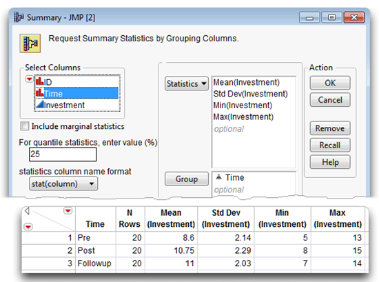
The value in the N Rows column is 20 for each variable—there are no missing values. The MIN(Investment) and MAX(Investment) values indicate no obvious errors in data. The Mean(Investment) score for Pre is 8.6, Post is 10.75, and Followup is 11.0.

A review of the group means shown in Figure 11.4 and Figure 11.5 suggests support for your study’s primary hypothesis, but does not appear to support the study’s secondary hypothesis. Notice that mean investment scores increase from the baseline survey at Time 1 (Pre) to the post-treatment survey at Time 2 (Post). If this increase is statistically significant, it would be consistent with your primary hypothesis that perceived investment increases immediately following the marriage encounter weekend.

However, notice that the mean investment scores remain at a relatively high level at the Time 3 (Followup), three weeks after the program. This trend is not consistent with your secondary hypothesis that the increase in perceived investment is short-lived.

However, at this point, you are only “eyeballing” the means. It is not clear whether any of the differences are statistically significant. To determine significance, you must analyze the data using a repeated-measures analysis. The next section shows a simple way to do this by using the Fit Y by X platform. Later sections show a repeated-measures ANOVA using the Fit Model platform.

Use the Fit Y by X Platform with a Matching Variable

One approach to analyze data from a simple repeated-measures design with no between-subject effects (grouping effects), is to do a one-way analysis of variance and use a matching variable to identify the repeating measures.

The Fit Y by X platform offers this feature.

Choose Fit Y by X from the Analyze menu.

Select Investment in the Select Columns list, and click Y, Response in the launch dialog. Select Time in the Select Columns list, and click X, Factor in the launch dialog.

Click OK to see the scatterplot of Investment by Time, which is the initial platform result.

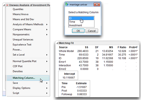
Choose the Matching Columns command from the menu on the Oneway Analysis title bar, as illustrated on the left in Figure 11.6. This command displays a dialog prompting you to select a matching variable.

When the Matching Columns dialog appears, choose ID as the matching variable. Click OK to see the analysis shown on the right in Figure 11.6.

When you choose a matching variable in the Fit Y by X one-way ANOVA platform, the analysis uses that variable to compute the within-subjects variation. With the within-subjects variation removed from the residual, the remaining error is the correct denominator to compute for the correct F statistic to test the repeated-measures between-subjects effect.

Figure 11.6: Fit Y by X Results of Matching Fit Analysis

Because the F statistic for the Time variable is significant (p < 0.0001), use the Compare Means option found on the menu on the Oneway Analysis title bar to see which of the means differ.

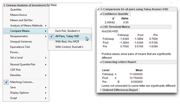
Return to the Oneway Analysis of Investment By Time results and select Compare Means > All Pairs, Tukey HSD from the menu on the title bar. The results of the multiple comparison tests are appended to the analysis and shown in Figure 11.7.

Note: This multiple comparison test does not consider the advantage of using the matching variable effect, and therefore gives a conservative result.

Keep in mind that the Fit Y by X platform can only be used for repeated measures analysis when there are no between-subject (grouping) effects, as in this example.

Figure 11.7: Compare Group Means with Tukey’s HSD

Steps to Interpret the Results

Step 1: Make sure the results look reasonable. Review all the results. First, check the number of observations given in the Summary table (N Rows in Figure 11.5). Next, check the number of levels for the response variable—the three levels of time show in the bar chart with the mean values above the bars (see Figure 11.4). Also, the Matching Fit report gives two degrees of freedom for the Time response variable, which is the number of levels (Pre, Post, and Followup) used in the analysis, minus 1 (3 – 1 = 2).

Step 2: Review the appropriate F statistic and its associated probability value. The first step to interpret the results of the analysis is to review the F-value of interest. The relevant F-value shows in the Matching Fit report for the Time variable (the within-subjects variable). This F-value tells whether to reject the null hypothesis that states,

“In the population, there is no difference in investment scores obtained at the three points in time.”

The hypothesis can be represented symbolically in this way:

H0: T1 = T2 = T3

where T1 is the baseline pre-weekend mean investment score, T2 is the mean score following the marriage encounter weekend, and T3 is the mean score three weeks after the marriage encounter weekend.

The Matching Fit report (shown again here) for the repeated-measures time variable gives a univariate F ratio that tests this null hypothesis. The F statistic for the Time effect is 30.28, with p < 0.0001. Because the p-value is less than 0.05, you can reject the null hypothesis of no difference in mean levels of commitment in the population. In other words, you conclude that there is an effect for the repeated-measures variable Time.

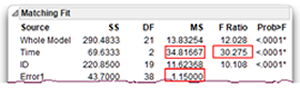
Computational note: This numerator for this statistic is the mean square for the Time effect (with 2 degrees of freedom). The denominator is the mean square for the error, labeled Error1 in the Matching Fit report (with 38 degrees of freedom). This is the appropriate denominator for the repeated measures F statistic because it does not include the between-subjects error. The F statistic is computed as 34.817 ÷ 1.105 = 30.275.

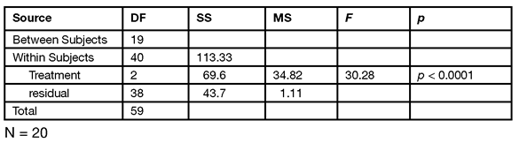
Step 3: Prepare your own version of an ANOVA table. The next step is to formulate the ANOVA summary table shown in Table 11.1. Note that the quantities needed for this table are either in the Matching Fit report or are easily computed:

• The ID variable in the report is the between-subjects effect with 19 DF.
• The within-subjects sum of squares (SS) and Mean Squares (MS) information is composed of the treatment (Time) effect and the within-subjects residual (Error1).
• The total within-subjects quantities are the sum of the treatment and residual terms.
• The total DF is the sum of the total within-subjects DF and the between-subjects DF.

Table 11.1: Repeated Measures ANOVA Table for Investment Study

Step 4: Review the results of contrasts. The significant effect for Time tells you that investment scores obtained at one point in time are significantly different from scores obtained from some other point in time. When you request Compare Means > All Pairs, Tukey HSD command, the means comparison results show at the bottom of the analysis report and comparison circles are shown to the right of the scatterplot. See the “Using JMP for Analysis of Variance” section in Chapter 8, “One-Way ANOVA with One Between-Subjects Factor,” for an explanation of comparison circles.

Options in the Means Comparisons report display the following results:

• The alpha value of 0.05 appears at the top of the report (see Figure 11.7).
• Next, a table of the actual absolute difference in the means minus the LSD. The Least Significant Difference (LSD) is the difference that would be significant. Pairs with a positive value are significantly different.

The Tukey letter grouping shows the mean scores for the three groups on the response variable (the Commitment variable in this study) and whether or not these group means are different at the 0.05 alpha level. You can see that the mean follow-up score is 11.0, the mean post-study score is 10.75, and the mean pre-study score is 8.6. The letter A identifies the follow-up score and the post-study score, and the letter B identifies the pre-study score. Therefore, you conclude that the pre-study mean score is significantly different from the post-study and follow-up mean scores, but the post-study and follow-up scores are not different.

Summarize the Results of the Analysis

The standard statistical interpretation format used for between-subjects ANOVA (as previously described in Chapter 8) is also appropriate for the repeated-measures design. The outline of this format appears again here.

A. Statement of the problem

B. Nature of the variables

C. Statistical test

D. Null hypothesis (Ho)

E. Alternative hypothesis (H1)

F. Obtained statistic

G. Obtained probability (p-value)

H. Conclusion regarding the null hypothesis

I. ANOVA summary table

J. Figure representing the results

Because most sections of this format are in previous chapters, they are not repeated here. Instead, the formal description of the results follows.

Formal Description of Results for a Paper

Mean investment size scores across the three trials are displayed in Figure 11.5. Results analyzed using one-way analysis of variance (anova) repeated-measures design revealed a significant effect for the treatment (time), with F(2,38) = 30.28; p < 0.0001. Contrasts showed that the baseline measure was significantly lower than the post-treatment and the follow-up mean scores. The post-treatment and follow-up means were not significantly different.

Repeated-Measures Design versus the Between-Subjects Design

An alternative to the repeated-measures design is a between-subjects design, as described in Chapter 8, “One-Way ANOVA with One Between-Subjects Factor.” For example, you could follow a between-subjects design and measure two groups immediately following the weekend program (at Time 2). In this between-subjects study, one group of couples attends the marriage encounter weekend and the other group does not attend the marriage encounter weekend. If you conduct the study well, you can then attribute any differences in the group means to the weekend experience.

In both the repeated-measures design and the between-subjects design, the sums of squares and mean squares are computed in the same way. However, an advantage of the repeated-measures design is that each participant also serves as a control. Because each participant serves in each treatment condition, variability in scores due to individual differences between participants is not a factor in determining the size of the treatment effect. The between-subjects variability is removed from the error term in the F test computation (see Table 11.1). This computation usually allows for a more sensitive test of treatment effects because the between-subjects variance can be much larger than the within-subject variance. This within-subject variance is smaller because multiple observations from the same participant tend to be positively correlated, especially when measured across time.

A repeated measures design also has the advantage of increased efficiency because this design requires only half the number of participants than needed in a between-subjects design. This can be an important consideration when the targeted study population is limited. These statistical and practical differences illustrate the importance of careful planning of the statistical analysis when designing an experiment.

Weaknesses of the One-Way Repeated Measures Design

The primary limitation of the present design is the lack of a control group. Because all participants receive the treatment in this design, there is no comparison that evaluates whether observed changes are the result of the experimental manipulation. For example, in the study just described, increases in investment scores might occur because of time spent together and have nothing to do with the specific program activities during the marriage encounter weekend (the treatment). Chapter 12, “Factorial ANOVA with Repeated-Measures Factors and Between-Subjects Factors,” shows how to remedy this weakness with the addition of an appropriate control group.

Another potential problem with this type of design is that participants might be affected by a treatment in a way that changes responses to subsequent measures. This problem is called a sequence effect and is discussed in the next section.

Sequence Effects

Another important consideration in a repeated-measures design is the potential for certain experimental confounds. In particular, the experimenter must control for order effects and carryover effects.

Order Effects

Order effects result when the ordinal position of the treatments biases participant responses. For example, suppose an experimenter studying perception requires participants to perform a reaction-time task in each of three conditions. Participants must depress a button on a response pad while waiting for a signal, and after receiving the signal they must depress a different button. The dependent variable is reaction time and the independent variable is the type of signal. The independent variable has three levels:

• condition 1—flash of light
• condition 2—an audio tone
• condition 3—both the light and tone simultaneously

Each test session consists of fifty trials. A mean reaction time is computed for each session. Assume that these conditions are presented in the same order for all participants (morning, before lunch, and after lunch).

The problem with this research design is that reaction-time scores can be adversely affected after lunch by fatigue. Responses to condition 3 might be more a measure of fatigue than a true treatment effect. Suppose the experiment yields mean scores for 10 participants as shown in Table 11.1. It appears that presentation of both signals (tone and light) causes a delayed reaction time compared to the other two treatments (tone alone or light alone).

Table 11.1: Mean Reaction Time (msecs) for All Treatment Conditions

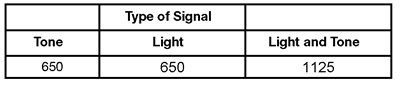
An alternative explanation for the preceding results is that a fatigue effect in the early afternoon causes the longer reaction times. According to this interpretation, you expect each of the three treatments to have longer reaction times if presented during the early afternoon period. If you collect the data as described, there is no way to determine which explanation is correct.

To control for this problem, you must vary the treatment order. This technique, called counterbalancing, presents the conditions in different orders to different participants. Table 11.2 shows a research design that uses counterbalancing.

Table 11.2: Counterbalanced Treatment Conditions to Control for Sequence Effects

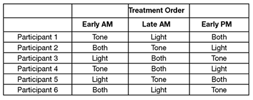
Note in Table 11.2 that each treatment occurs an equal number of times at each point of measurement. To achieve complete counterbalancing, you must use each combination of treatment sequences for an equal number of participants.

Complete counterbalancing becomes impractical as the number of treatment conditions increases. For example, there are only 6 possible sequences of 3 treatments, but this increases to 24 sequences with 4 treatments, 120 sequences with 5 treatments, and so forth. Usually, counterbalancing is possible only if the independent variable assumes a relatively small number of values.

Carryover Effects

Carryover effects occur when an effect from one treatment changes (carries over to) the participants’ responses in the following treatment condition. For example, suppose you investigate the sleep-inducing effect of three different drugs. Drug 1 is given on night 1 and sleep onset latency is measured by electroencephalogram. The same measure is collected on nights 2 and 3, when drugs 2 and 3 are administered. If drug 1 has a long half-life, then it can still exert an effect on sleep latency at night 2. This carryover effect makes it impossible to accurately assess the effect of drug 2.

To avoid potential carryover effects, the experimenter can separate the experimental conditions by some period of time, such as one week. Counterbalancing also provides some control over carryover effects. If all treatment combinations can be given, then each treatment will be followed (and preceded) by each other treatment with equal frequency. However, counterbalancing is more likely to correct order effects than carryover effects. Counterbalancing is advantageous because it enables the experimenter to measure the extent of carryover effects and to make appropriate adjustments to the analysis.

Ideally, careful consideration of experimental design allows the experimenter to avoid significant carryover effects in a study. This is another consideration in choosing between a repeated-measures and a between-subjects design. In the study of drug effects described above, the investigator can avoid any possible carryover effects by using a between-subjects design. In that design, each participant only receives one of the drug treatments.

Univariate or Multivariate ANOVA for Repeated-Measures Analysis?

The analysis described previously in the “A Univariate Approach for Repeated-Measures Analysis Using the Fit Y by X Platform” section was conducted as a conventional univariate repeated-measures ANOVA. However, using the univariate approach requires that the data fulfill two assumptions:

• The scores from experimental treatments have a multivariate normal distribution in the population. Normality is impossible to prove but becomes more likely as sample size increases.
• The common covariance matrix has a specific type of pattern called sphericity (homogeneity of covariance).

Homogeneity of covariance refers to the covariance between participants for any two treatments. One way to conceptualize this is that participants should have the same rankings in scores for all pairs of levels of the independent variable. For example, if there are three treatment conditions (T1, T2, and T3), the covariance between T1 and T2 should be comparable to the covariance between T2 and T3, and to the covariance between T1 and T3. Homogeneity of covariance is sufficient for test validity, but a less specific type of covariance pattern, called sphericity, is a necessary condition for the validity of a univariate analysis of a repeated-measures design (Huynh and Mandeville, 1979, Rouanet and Lepine, 1970).

The violation of homogeneity of covariance (sphericity) is particularly problematic for repeated-measures designs. In the case of between-subject designs, the analysis still produces a robust F test even when this assumption is not met (provided sample sizes are equal). On the other hand, a violation of this assumption with a repeated-measures design leads to an increased probability of a Type I error (rejection of a true null hypothesis). Therefore, you must take greater care when analyzing repeated-measures designs to either prove that the assumptions of the test have been met or alter the analysis to account for the effects of the violation.

For a more detailed discussion of the validity conditions for the univariate ANOVA and alternative approaches to the analysis of repeated measures data, see Barcikowski and Robey (1984) or LaTour and Miniard (1983).

The next section approaches repeated-measures analysis as a multivariate problem, and tests sphericity for this marriage data example.

Review the Data Table for a Multivariate Analysis

As previously described, the sample consists of data from the 20 married women who participated in the marriage encounter program. The response variable is the size of the investment the participants (the wives) believe they have made in their relationships. Investment size is measured by a scale that gives a continuous numeric value.

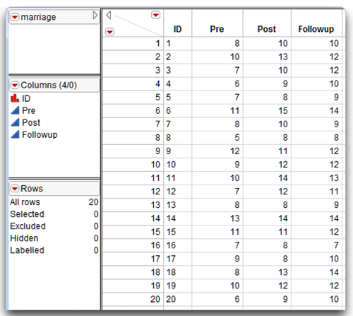
The JMP data table called Marriage.jmp lists the investment scores obtained at the three different points in time arranged as three columns. The nominal variable called ID identifies each couple. The investment score variable Pre lists the investment scores recorded at Time 1, Post records the scores at Time 2, and Followup records the scores at Time 3 (see Figure 11.8). The nominal variable called ID identifies each couple.

Figure 11.8: Listing of Data for Multivariate Repeated-Measures Analysis

Using the Fit Model Platform for Repeated-Measures Analysis

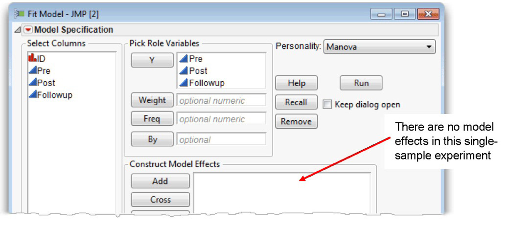
The Fit Model platform can analyze repeated-measures data using multivariate methods (MANOVA). The three commitment measurements (Pre, Post, and Followup) are three response variables and the fitting personality is Manova. In a between-subjects study, the predictor variable (or model effect) appears in the Model Effects area of the Fit Model dialog. The Fit Model dialog in Figure 11.9 is similar to the one shown in Chapter 10, “Multivariate Analysis of Variance (MANOVA) with One Between-Subjects Factor,” except there is no model effect.

Figure 11.9: Fit Model Dialog for Multivariate Repeated-Measures Analysis

When you click Run in the Fit Model dialog, the initial multivariate analysis appears, as shown on the left in Figure 11.10. This initial result plots the means of the three response variables, which again indicates the difference between the Pre and Post scores, but shows little difference between the Post and Followup scores.

To continue with the repeated-measures analysis,

Click the Univariate Tests Also check box. This option gives the sphericity test and univariate analysis of the data.

Click the Test Each Column Separately Also check box. This option sets up contrasts between the Pre and Post mean scores, and between the Pre and Followup mean scores.

Choose Repeated Measures from the Choose Response menu, as shown in Figure 11.10.

Because the measures are repeated, an additional dialog prompts for a name to call the repeated measure variable. The default name is Time, which is a typical type of repeated measures, and appropriate for this example.

Click OK in the Specification of Repeated Measures dialog to see the completed analysis.

Figure 11.10: Initial MANOVA Results for Repeated Measures Analysis

Note: Most JMP results include tables, charts, statistics and other statistical tools geared for any possible request or model you might specify. This is especially true for the MANOVA reports because they are equipped to handle complex situations. However, the example in this chapter is very simple, and only requires that you look at a single line of results. The figures in this chapter show unneeded outline nodes as closed in the analysis and open only what you need to see.

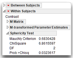
Examine the Sphericity Text

The MANOVA results include both univariate and multivariate F tests for the within-subjects time effect. To decide which test to use, look at the Sphericity Test table, which is the first table in the Within Subjects section, as shown here. The sphericity test, called Mauchey’s criterion, has a significant F test with a p-value (prob > Chisq) of 0.0323. This marginally significant test suggests the data display a significant departure from sphericity. In other words, you reject the null hypothesis of the homogeneity of covariance. However, this test is very sensitive and any deviation from sphericity results in a significant F test. You can compensate for small to moderate deviations from sphericity through use of a modified F test, or if there is a severe departure from sphericity (p < 0.0001), then multivariate tests should be used.

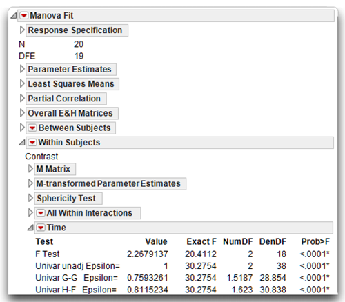
Examine the Multivariate Analysis of Variance

Figure 11.11 shows the results of the repeated measures analysis for the time effect. The line in the Time report labeled Univar unadj Epsilon gives the Exact F as 30.2754 with 2 degrees of freedom in the numerator and 38 degrees of freedom in the denominator. This is the same univariate analysis given by the Fit Y by X platform shown previously. However, to account for the deviation in sphericity, you can refer to the modified F tests or to the multivariate F test, which is also given in the Time report.

The primary concern when the sphericity pattern is not present is that theF test will be too liberal and lead to inappropriate rejection of the null hypothesis (Type I error). Modifications to compensate for non-sphericity make the test more conservative.

The currently accepted method to modify the F test to account for deviations from sphericity is to reduce the degrees of freedom in the numerator and the denominator associated with the F-value by some fraction epsilon (ε). Greenhouse and Geisser (1959) offer a technique for estimating the epsilon degrees-of-freedom adjustment. The degrees of freedom are multiplied by the correction factor to yield a number that is either lower or unchanged. Therefore, a given test has fewer degrees of freedom and requires a greater Fvalue to achieve a given p level. With epsilon at a value of 1 (meaning the assumption has been met), the degrees of freedom are unchanged. To the extent that sphericity is not present, epsilon is reduced and this further decreases the degrees of freedom to produce a more conservative test.

The computations for the G-G epsilon are performed by the MANOVA when you check Univariate Tests Also in the initial dialog (see Figure 11.10). An even more conservative adjustment, called the Huynh-Feldt or H-F epsilon (Huynh and Feldt, 1970), is also included.

Although the exact procedure to follow depends somewhat on characteristics specific to a given data set, there is some consensus for use of the following general guidelines:

• Use the adjusted univariate test when the Greenhouse-Geisser (G-G) epsilon value is greater than or equal to 0.75.
• If the G-G epsilon is less than 0.75, a multivariate analysis (MANOVA) is a more powerful test.

A G-G epsilon value of 0.759, which is shown in Figure 11.11, suggests using the adjusted univariate F test (F = 30.28, p < 0.0001) or the multivariate F test, which is discussed next.

Figure 11.11: Repeated Measures Analysis of Time

Note: Don’t forget that the Time variable on the multivariate report is the repeated measures variable constructed from the Pre, Post, and Followup variables in the data.

The Multivariate F Test

As a repeated-measures design consists of within-subjects observations across treatment conditions, the individual treatment measures can be viewed as separate, correlated dependent variables. The data is easily conceptualized as multivariate even though the design is univariate, and it can be analyzed with multivariate statistics. In this type of analysis, each level of the repeated factor is treated as a separate variable. The first line in the Time report, which is shown in Figure 11.11, gives the multivariate F-value of 20.4112, with p < 0.0001.

The MANOVA test has an advantage over the univariate test in that it requires no assumption of sphericity. Some statisticians recommend that the MANOVA be used frequently, if not routinely, with repeated-measure designs (Davidson, 1972). This argument is made for several reasons.

In selecting a test statistic, it is always desirable to choose the most powerful test. A test is said to have power when it is able to correctly reject the null hypothesis. In many situations, the univariate ANOVA is more powerful than the MANOVA and is therefore the better choice if the sphericity assumptions are met. However, the test for sphericity is not very powerful with small samples. Therefore, only when the n is large (20 greater than the number of treatment levels or n > k + 20) does the test for sphericity have sufficient power. Remember that the multivariate test becomes just as powerful as the univariate test as the n grows larger. However, keep in mind that with a small n there is no certainty that the assumptions underlying the univariate MANOVA have been met, but with a large n the MANOVA is equally if not more powerful than the univariate test.

Others argue that the univariate approach offers a more powerful test for many types of data and should not be so readily abandoned. Tabachnick and Fidell (2001) feel that the MANOVA should be reserved for those situations that cannot be analyzed with the univariate ANOVA.

With the current example, the sample is composed of 20 participants and falls below the sensitivity threshold for sphericity tests described above (n < k + 20). In other words, the decision to reject the null hypothesis of significant departure from the homogeneity of variance assumption (Mauchly’s criterion of 0.683, p < 0.05) might not be correct. Fortunately, the standard F, adjusted F-values, and the multivariate statistics suggest rejection of the study’s null hypothesis of no difference in investment scores across the three points in time.

To interpret the multivariate results, follow the same steps outlined previously.

Steps to Review the Results

Step 1: Make sure that everything looks reasonable. First, check the number of observations listed with the initial analysis in the Response Specification dialog to make certain data from all participants is included in the analysis. If any data are missing, then all data for that participant is automatically dropped from the analysis. Next, check the number of levels assigned to the response variable—there are three levels of Time in the means plot with the means listed beneath it (Figure 11.10).

Step 2: Review the appropriate F statistic and its associated probability value. The first step in interpreting the results of the analysis is to review the F-value and associated statistics. The relevant F-value shows in the Time report for the Within Subjects section of the analysis. This F-value tells you whether to reject the null hypothesis that states,

“In the population, there is no difference in investment scores obtained at the three points in time.”

This hypothesis can be represented symbolically in this way:

H0: T1 = T2 = T3

where T1 is the baseline pre-weekend mean investment score, T2 is the mean score following the marriage encounter weekend, and T3 is the mean score three weeks after the marriage encounter weekend.

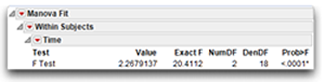
The report for the repeated measures Time variable, shown again here, gives the multi- variate F ratio that tests this null hypothesis. The exact F of 20.4112 with 2 and 18 degrees of freedom has a significant probability of less than 0.0001. This F statistic is significant because its p-value is less than 0.05 so you can reject the null hypothesis of no differences in mean levels of commitment in the population. In other words, you conclude that there is an effect for the repeated-measures variable, Time.

Step 3: Review the contrast results. The significant effect for Time tells you that investment scores obtained at one point in time are significantly different from scores obtained at some other point in time. You still do not know which scores significantly differ. To determine this, consult the planned comparisons given when you check Test Each Column Separately Also on the initial multivariate results dialog (see Figure 11.10). By default, this option sets up contrasts between the first and second time scores (Pre and Post mean scores), and between the first and third time scores (Pre and Followup mean scores). Figure 11.12 shows these results.

Figure 11.12: Results of Contrasts Given by the Fit Model MANOVA

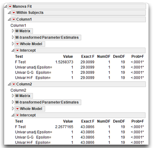
The contrast between the Pre and Post mean scores evaluates the primary hypothesis that investment increases significantly after the marriage intervention at post-treatment (Time 2) compared to baseline (Time 1).

The multivariate F ratio for this contrast is found in the table labeled Intercept, in the Column 1 report. You can see that the obtained F-value is 29.0099. It has 1 and 19 degrees of freedom and is significant at p < 0.0001. This F test supports the primary hypothesis that investment scores display a significant increase from Time 1 to Time 2 as illustrated by the plot in the initial MANOVA results shown in Figure 11.10.

The contrast that compares the baseline scores (Pre) to the follow-up scores taken three weeks after the marriage encounter shows in the Intercept table in the Column 2 report. The F-value for this contrast is also statistically significant (p < 0.0001), which indicates that these two treatment means are different. Inspection of the means in Figure 11.10 shows that the follow-up mean is greater than the baseline mean. The second hypothesis stated that there would not be an increase in investment scores Time 1 (Pre) and Time 3 (Followup). The significant contrast does not support this hypothesis of no change. The increase in perceived investment size is maintained three weeks after the marriage encounter.

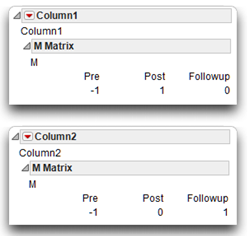
The contrast reports have generic labels, Column1 and Column2, denoting the first contrast and the second contrast. The contrast variables can be seen by looking at the M matrix for each contrast, as shown here. In each case, the contrasts are identified by the set of weights (–1 and 1) that sum to zero. In a repeated-measures analysis, the first response variable listed in the Fit Model dialog always acts as the baseline measure.

The contrast result tables are labeled Intercept because the estimate of a group mean in a simple means comparison is its Y intercept.

Summarize the Results of the Analysis

The standard statistical interpretation format used for between-subjects ANOVA (as previously described in Chapter 8) is also appropriate for the repeated-measures design. The outline of this format appears again here:

A. Statement of the problem

K. Nature of the variables

L. Statistical test

M. Null hypothesis (Ho)

N. Alternative hypothesis (H1)

O. Obtained statistic

P. Obtained probability (p-value)

Q. Conclusion regarding the null hypothesis

R. ANOVA summary table

S. Figure representing the results

Because most sections of this format appear in previous chapters, they are not repeated here. Instead, the formal description of the results follows.

Formal Description of Results for a Paper

Mean investment size scores across the three trials are displayed in Figure 11.4. Results analyzed using a one-way analysis of variance (ANOVA) repeated-measures design revealed a significant effect for the treatment (Time), with F(2,18) = 20.4112; p < 0.0001. Contrasts showed that the baseline measure was significantly lower than the post-treatment trial, F(1,19) = 29.0099, p < 0.0001, and the follow-up trial, F(1,19) = 43.0866; p < 0.0001.

Summary

You can use the one-way repeated-measures ANOVA to analyze data from studies in which each participant is exposed to every level of the independent variable. In some cases, this involves a single-group design in which repeated measurements are taken at different points in time. Single-group repeated-measures studies often suffer from a number of problems. Adding a second group of participants (a control group) to the design rectifies some of these problems. The next chapter shows how to analyze data from a study with two groups.

Appendix: Assumptions of the Multivariate Analysis of Design with One Repeated-Measures Factor

Level of measurement

Repeated-measures designs are so-named because they normally involve obtaining repeated measures on some response variable from a single sample of participants. This response variable should be assessed on an interval-level or ratio-level of measurement. The predictor variable should be a nominal-level variable (a categorical variable), which typically codes “time,” “trial,” “treatment,” or some similar construct.

Independent observations

A given participant’s score in any one condition should not be affected by any other participant’s score in any of the study’s conditions. However, it is acceptable for a given participant’s score in one condition to be dependent upon his or her own score in a different condition. This is another way of saying, for example, that it is acceptable for participants’ scores in condition 1 to be correlated with their scores in condition 2 or condition 3.

Random sampling

Scores on the response variable should represent a random sample drawn from the populations of interest.

Multivariate normality

The measurements obtained from participants should follow a multivariate normal distribution. Under conditions normally encountered in social science research, violations of this assumption have only a very small effect on the Type I error rate (the probability of incorrectly rejecting a true null hypothesis).

References

Barcikowski, R., and Robey, R. 1984. “Decisions in Single Group Repeated Measures Analysis: Statistical Tests and Three Computer Packages.” The American Statistician, 38, 148–150.

Davidson, M. 1972. “Univariate versus Multivariate Tests in Repeated-Measures Experiments.” Psychological Bulletin, 77, 446–452.

Greenhouse, S., and Geisser, S. 1970. “On Methods in the Analysis of Profile Data.” Psychometrika, 24, 95–112.

Huynh, H., and Feldt, L. S. 1970. “Conditions Under Which Mean Square Ratios in Repeated Measurements Designs Have Exact F-Distributions.” Journal of the American Statistical Association, 65, 1582–1589.

Huynh, H., and Mandeville, G. 1979. “Validity Conditions in Repeated Measures Designs.” Psychological Bulletin, 86,964–973.

Kashy, D. A., and Snyder, D. K. 1995. “Measurement and Data Analytic Issues in Couples Research.” Psychological Assessment, 7, 338–348.

LaTour, S., and Miniard, P. 1983. “The Misuse of Repeated Measures Analysis in Marketing Research.” Journal of Marketing Research, 20, 45–57.

Olson, C. 1976. “On Choosing a Test Statistic in Multivariate Analysis of Variance.” Psychological Bulletin, 83, 579–586.

Rouanet, H., and Lepine, D. 1970. “Comparison between Treatments in a Repeated-Measurement Design: ANOVA and Multivariate Methods.” The British Journal of Mathematical and Statistical Psychology, 23, 147–163.

Rusbult, C. E. 1980. “Commitment and Satisfaction in Romantic Associations: A Test of the Investment Model.” Journal of Experimental Social Psychology, 16, 172–186.

SAS Institute Inc. 2012. Modeling and Multivariate Methods. Cary, NC: SAS Institute Inc.

Tabachnick, B. G., and Fidell, L. S. 2001. Using Multivariate Statistics, Fourth Edition. New York: Harper Collins.