
 6
6
Assessing Scale Reliability with Coefficient Alpha
Overview
This chapter shows how to use the Multivariate platform in JMP to compute the coefficient alpha reliability index (Cronbach’s alpha) for a multiple-item scale. It reviews basic issues regarding the assessment of reliability, and describes the circumstances under which a measure of internal consistency is likely to be high. Fictitious questionnaire data are analyzed to demonstrate how you can perform an item analysis to improve the reliability of scale responses.
Introduction: The Basics of Scale Reliability
Example of a Summated Rating Scale
True Scores and Measurement Error
Underlying Constructs versus Observed Variables
Cronbach’s Alpha for the 4-Item Scale
Method to Compute Item-Total Correlation
Cronbach’s Alpha for the 3-Item Scale
Introduction: The Basics of Scale Reliability
You can compute coefficient alpha, also called Cronbach’s alpha, when you have administered a multiple-item rating scale to a group of participants and want to determine the internal consistency of responses to the scale. The items constituting the scale can be scored dichotomously, such as “right” or “wrong.” Or, items can use a multiple-point rating format—participants can respond to each item using a 7-point “agree–disagree” rating scale.
This chapter shows how to use the Multivariate platform in JMP to compute the coefficient alpha for the types of scales often used in social science research and surveys in general. However, this chapter will not show how to actually develop a multiple-item scale for use in research. To learn about recommended approaches for creating summated rating scales, see Spector (1992).
Example of a Summated Rating Scale
A summated rating scale consists of a short list of statements, questions, or other items to which participants respond. Often, the items that constitute the scale are statements, and participants indicate the extent to which they agree or disagree with each statement by selecting some response on a rating scale, such as a 7-point rating scale in which 1 = “Strongly Disagree” and 7 = “Strongly Agree”). The scale is called a summated scale because the researcher can sum responses to all selected responses to create an overall score on the scale. These scales are often referred to as Likert-type scales.
Note: Likert scale items can be averaged to give a response instead of summed. Using the mean response eliminates the problem of non-response and is sometimes easier to interpret than the sum of the responses.
As an example, imagine that you are interested in measuring job satisfaction in a sample of employees. To do this, you might develop a 10-item scale that includes items such as “in general, I am satisfied with my job.” Employees respond to these items using a 7-point response format in which 1 = “Strongly Disagree” and 7 = “Strongly Agree.”
You administer this scale to 200 employees and compute a job satisfaction score by summing each employee’s responses to the 10 items. Scores can range from a low of 10 (if the employee circled “Strongly Disagree” for each item) to a high of 70 (if the employee circled “Strongly Agree” for each item). You hope to use job satisfaction scores as a predictor variable in research. However, the people who later read about your research have questions about the psychometric properties of scale responses. At the very least, you need to show empirical evidence that responses to the scale are reliable. This chapter discusses the meaning of scale reliability and shows how to use JMP to obtain an index of internal consistency for summated rating scales.
True Scores and Measurement Error
Most observed variables measured in the social sciences (such as scores on your job satisfaction scale) consist of two components:
- A true score that indicates where the participant actually stands on the variable of interest.
- Measurement error, which is a part of almost all observed variables, even those variables that seem to be objectively measured.
Imagine that you assess an observed variable, age, in a group of participants by asking them to indicate their age in years. To a large extent, this observed variable (what the participants wrote down) is influenced by the true score component. That is, the participant’s response is influenced by how old they actually are. Unfortunately, this observed variable is also be influenced by measurement error. Some participants write down the wrong age because they don’t know how old they are, some will write the wrong age because they don’t want the researcher to know how old they are, and other participants write the wrong age because they didn’t understand the question. In short, it is likely that there will not be a perfect correlation between the observed variable (what the participants write down) and their true age scores.
Measurement error can occur even though the age variable is relatively objective and straightforward. If this simple a question can be influenced by measurement error, imagine how much more error results when more subjective constructs, such as the items that constitute your job satisfaction scale, are measured.
Underlying Constructs versus Observed Variables
In applied research, it is useful to draw a distinction between underlying constructs versus observed variables.
- An underlying construct is the hypothetical variable that you want to measure. In the job satisfaction study, for example, you want to measure the underlying construct of job satisfaction within a group of employees.
- The observed variable consists of the responses you actually obtain. In this example, the observed variable consisted of scores on the 10-item measure of job satisfaction. These scores might or might not be a good measure of the underlying construct.
Reliability Defined
With this understanding, it is now possible to provide some definitions. A reliability coefficient can be defined as the percent of variance in an observed variable that is accounted for by true scores on the underlying construct. For example, imagine that, in the study just described, you were able to obtain two scores for the 200 employees in the sample—their observed scores on the job satisfaction questionnaire and their true scores on the underlying construct of job satisfaction. Assume that you compute the correlation between these two variables. The square of this correlation coefficient represents the reliability responses to your job satisfaction scale. It is the percent of variance in observed job satisfaction scores accounted for by true scores on the underlying construct of job satisfaction.
The preceding was a technical definition for reliability, but this definition is of little use in practice because it is usually not possible to obtain true scores for a variable. For this reason, reliability is often defined in terms of the consistency of the scores obtained on the observed variable. An instrument is said to be reliable if it is shown to provide consistent scores upon repeated administration, upon administration by alternate forms, and so forth. A variety of methods to estimate scale reliability are used in practice.
Test-Retest Reliability
Assume that you administer your measure of job satisfaction to a group of 200 employees, first in January and again in March. If the instrument is reliable, you expect that the participants who provided high scores in January will tend to provide high scores again in March, and that those with low scores in January will also have low scores in March. These results support the test-retest reliability of responses to the scale. You assess test-retest reliability by administering the same instrument to the same sample of participants at two points in time, and then computing the correlation between sets of scores.
But what is an appropriate interval over which questionnaires should be administered? Unfortunately, there is no hard-and-fast rule of thumb here. The interval depends on what is being measured. For enduring constructs such as personality variables, test-retest reliability has been assessed over several decades. For other constructs such as depressive symptomatology, the interval tends to be much shorter due to the fluctuating course of depression and its symptoms. Generally speaking, the test-retest interval should not be so short that respondents recall their responses to specific items (less than a week) but not so long as to measure natural variability in the construct (real change in depressive symptoms). The former leads to an overstatement of test-retest reliability, whereas the latter leads to understatement of test-retest reliability.
Internal Consistency
Another important aspect of reliability is internal consistency. Internal consistency is the extent to which the individual items that constitute a test correlate with one another or with the test total.
Internal consistency and test-retest procedures measure different aspects of scale reliability estimation. That is, internal consistency evaluation is not an alternative to test-retest measures. For example, some constructs, such as mood measures, do not typically exhibit test-retest reliability, but should show internal consistency.
In the social sciences, a widely used index of internal consistency is the coefficient alpha or Cronbach’s alpha (Cronbach, 1951), which is symbolized by the Greek letter α.
Cronbach’s Alpha
Cronbach’s alpha is a general formula for scale reliability based on internal consistency. It gives the lowest estimate of reliability that can be expected for an instrument.
The formula for coefficient alpha is
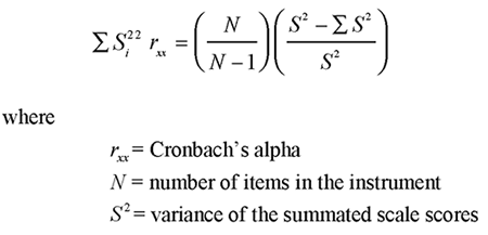
That is, assume that you compute a total score for each participant by summing responses to the scale. The variance of this total score variable is S2.
![]() = the sum of the variances of the individual items that constitute this scale.
= the sum of the variances of the individual items that constitute this scale.
Other factors held constant, Cronbach’s alpha is high when there are many highly correlated items in the scale. To understand why Cronbach’s alpha is high when the items are highly correlated with one another, consider the second term in the preceding formula:
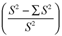
This term shows that the variance of the summated scales scores, S2, is divided by itself to compute Cronbach’s alpha. However, the combined variance of the individual items is first subtracted from this variance before the division is performed. This part of the equation shows that as the combined variance of the individual items becomes small, Cronbach’s alpha becomes larger.
This is important because (with other factors held constant), stronger correlations between the individual items give a smaller ![]() term. Thus, Cronbach’s alpha for responses to a given scale is likely to be large to the extent that the variables constituting that scale are strongly correlated.
term. Thus, Cronbach’s alpha for responses to a given scale is likely to be large to the extent that the variables constituting that scale are strongly correlated.
Computing Cronbach’s Alpha
Imagine that you have conducted research in the area of prosocial behavior and have developed an instrument designed to measure two separate underlying constructs: helping others and financial giving.
- Helping others refers to prosocial activities performed to help coworkers, relatives, and friends.
- Financial giving refers to giving money to charities or the homeless.
See Chapter 14: “Principal Component Analysis,” for a more detailed description of these constructs. In the following questionnaire, items 1 to 3 are designed to assess helping others, and items 4 to 6 are designed to assess financial giving.
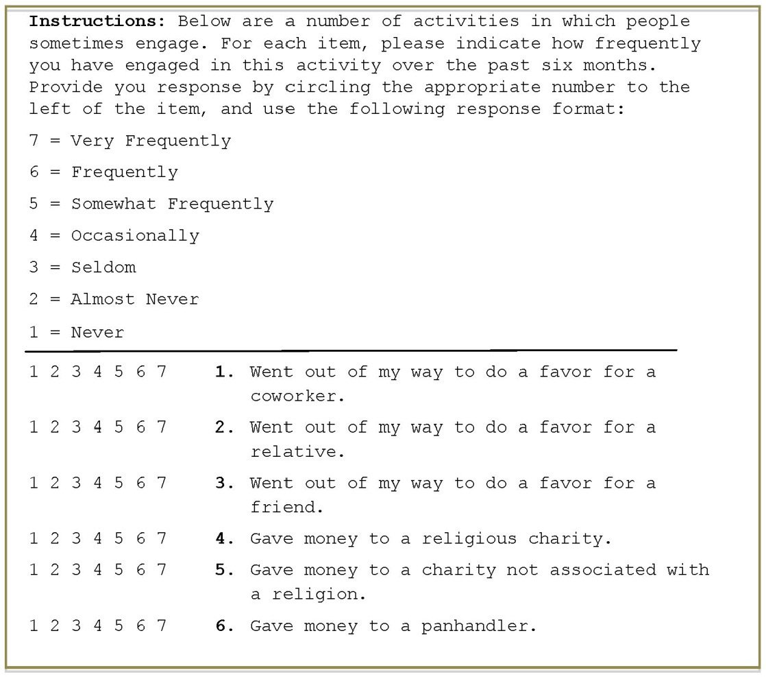
Assume that you have administered this 6-item questionnaire to 50 participants. For the moment, consider only the reliability of the scale that includes items 1 to 3 (the items that assess helping others).
Further assume that you made a mistake in assessing the reliability of this scale. Suppose you erroneously believed that the “helping others” construct was assessed by items 1 to 4 (whereas, in reality, that construct was assessed by items 1 to 3). It is instructive to see what happens when you mistakenly include item 4 in the analysis. The next section looks at this 4-item scale.
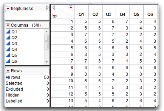
This example uses the JMP data table called helpfulness.jmp. Figure 6.1 shows a partial listing of the data. Ordinarily, you would not compute Cronbach’s alpha in this case because internal consistency is often underestimated with so few items. Cronbach’s alpha also tends to overestimate the internal consistency of responses to scales with 40 or more items (Cortina, 1993; Henson, 2001).
The JMP Multivariate Platform
In JMP, the Multivariate platform gives simple statistics and correlations and, optionally, can compute Cronbach’s alpha (internal consistency) for a summated rating scale.
![]() Open the helpfulness data table. Note that the items are called Q1–Q6, and each row is the set of responses given by the 50 participants.
Open the helpfulness data table. Note that the items are called Q1–Q6, and each row is the set of responses given by the 50 participants.
Figure 6.1: Partial Listing of the Helpfulness Survey Data Table
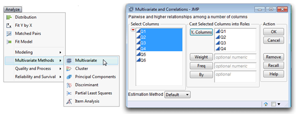
![]() On the Analysis main menu, the Multivariate Methods command has several platforms. For this example, choose Analysis > Multivariate Methods > Multivariate.
On the Analysis main menu, the Multivariate Methods command has several platforms. For this example, choose Analysis > Multivariate Methods > Multivariate.
![]() When the launch dialog appears, select Q1, Q2, Q3, and Q4 as analysis (Y) variables, as shown in Figure 6.2.
When the launch dialog appears, select Q1, Q2, Q3, and Q4 as analysis (Y) variables, as shown in Figure 6.2.
Figure 6.2: Multivariate Command and Launch Dialog
Click OK in the launch dialog to see the initial results. By default, the initial multivariate platform results show a Correlations table and a bivariate scatterplot matrix with a density ellipse for each pair of Y variables.
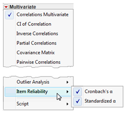
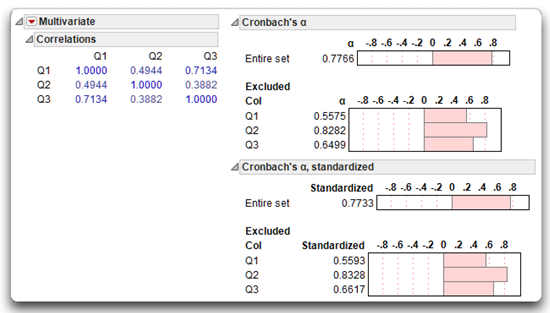
![]() Use options from the red triangle menu on the Multivariate title bar to see the results in Figure 6.3. That is, turn off (uncheck) Scatterplot Matrix, and select both Cronbach’s Alpha and Standardized Alpha from the Item Reliability submenu, as shown here.
Use options from the red triangle menu on the Multivariate title bar to see the results in Figure 6.3. That is, turn off (uncheck) Scatterplot Matrix, and select both Cronbach’s Alpha and Standardized Alpha from the Item Reliability submenu, as shown here.
Cronbach’s Alpha for the 4-Item Scale
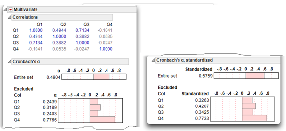
Figure 6.3 shows the Cronbach’s alpha computations. The Cronbach’s alpha for the nonstandardized set, noted as the entire set on the report, is only 0.4904. This is the reliability coefficient for items Q1 to Q4. This reliability coefficient is often reported in published articles.
How Large Is an Acceptable Reliability Coefficient?
Nunnally (1978) suggests that 0.70 is an acceptable reliability coefficient. Reliability coefficients less than 0.70 are generally seen as inadequate. However, you should remember that this is only a rule of thumb and scientists sometimes report a coefficient alpha (Cronbach’s alpha) under 0.70 (and sometimes even under 0.60).
Also, a larger alpha coefficient is not necessarily always better than a smaller one. An ideal estimate of internal consistency is thought to be between 0.80 and 0.90 (Clark and Watson, 1995; DeVellis, 1991) because estimates in excess of 0.90 suggest item redundancy or inordinate scale length.
Alpha Comparison for Item Selection
The coefficient alpha of 0.49 reported in Figure 6.3 is not acceptable. In some situations, the reliability of responses to a multiple-item scale improves by dropping a redundant item. One useful way to evaluate an item and determine if it should be deleted is to compare its α with the α for the entire set. The rule of thumb is that if an item α is greater than the overall α that includes the item, then scale reliability improves when that item is dropped from the set.
For example, the Excluded Col section of the Chronbach’s alpha reports show the Q4 alpha value to be 0.7766, which is considerable larger than the Entire Set value of 0.4904. Likewise, the standardized alpha for Q4 is 0.7733 and the overall standardized alpha is 0.5797. These comparisons indicate that Q4 should be dropped from the analysis. Coefficient alpha computations revealed that Q4 was accidentally included in this initial example.
Figure 6.3: Multivariate Results Showing Correlations and Cronbach’s Alpha
Item-Total Correlations
In some situations, the reliability of responses to a multiple-item scale improves by deleting those items with poor item-total correlations.
An item-total correlation is the correlation between an individual item and the sum of the remaining items that constitute the scale.
A small item-total correlation is evidence that the item is not measuring the same construct measured by the other scale items. This means that you could choose to discard items that show small item-total correlations. The next section shows how to compute item-total correlations.
Method to Compute Item-Total Correlation
JMP version 10 does not automatically compute item-total correlations. However, there are several ways to construct item-total correlations using JMP features. This section shows how to use the data table and formulas, followed by the Multivariate platform to look at item-total correlations.
Begin by constructing four new variables in the helpfulness data table. Each new variable is the sum of three original variables. There is a sum column for each combination of three original variables.
![]() Use the Add Multiple Columns command from the Cols main menu to add four numeric columns to the data table.
Use the Add Multiple Columns command from the Cols main menu to add four numeric columns to the data table.
![]() Give the columns convenient names that identify their formulas, such as Q2+Q3+Q4, Q1+Q3+Q4, Q1+Q2+Q4, and Q1+Q2+Q3.
Give the columns convenient names that identify their formulas, such as Q2+Q3+Q4, Q1+Q3+Q4, Q1+Q2+Q4, and Q1+Q2+Q3.
![]() For each new column, use its formula editor to compute column values. To do this, right-click in the column name area and select Formula from the popup menu, as shown in Figure 6.4. Or, highlight the column and choose Formula from the Cols menu. When the formula editor appears, enter the formula identified by the column name.
For each new column, use its formula editor to compute column values. To do this, right-click in the column name area and select Formula from the popup menu, as shown in Figure 6.4. Or, highlight the column and choose Formula from the Cols menu. When the formula editor appears, enter the formula identified by the column name.
See the “Compute Column Values with a Formula” section in Chapter 3, “Working with JMP Data,” for a detailed example of how to use the JMP Formula Editor.
Figure 6.4: Create Columns and Compute Sums
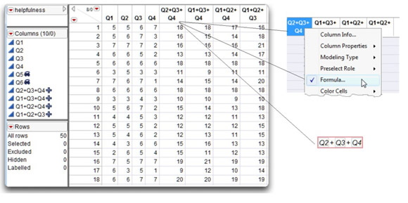
Note: The Helpfulness data table includes these computed variables. In Figure 6.4, the Q5 and Q6 variables are hidden and do not show in the data table.
Use the Multivariate platform to compute correlations between the original variables and the constructed sums.
![]() Choose Multivariate Methods > Multivariate from the Analyze menu.
Choose Multivariate Methods > Multivariate from the Analyze menu.
![]() In the Multivariate launch dialog, select Q1–Q4 and the four sum variables in the Select Columns list and click Y, Columns on the dialog. The completed dialog should look like the one shown at the top in Figure 6.5.
In the Multivariate launch dialog, select Q1–Q4 and the four sum variables in the Select Columns list and click Y, Columns on the dialog. The completed dialog should look like the one shown at the top in Figure 6.5.
![]() Click OK in the launch dialog to see the results shown at the bottom in Figure 6.5.
Click OK in the launch dialog to see the results shown at the bottom in Figure 6.5.
Figure 6.5: Item-Total Correlations for Each Item
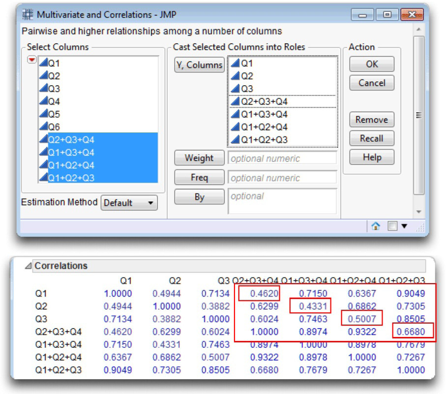
The item-total correlations now show in the Correlations table. You only need to look at the portion of the table shown boxed in Figure 6.5. The item-total correlations are the diagonal quantities. For example, to see the correlation between Q1 and the sum of Q2, Q3, and Q4, look at the intersection of the row labeled Q1 and the column labeled Q2+A3+Q4.
You can see that items 1 to 3 demonstrate reasonably strong correlations with the sum of the remaining items on the scale. However, item Q4 demonstrates an item-total correlation of approximately –0.037, which suggests that item Q4 is not measuring the same construct as items Q1 to Q3.
Cronbach’s Alpha for the 3-Item Scale
Now look at the alpha computations for the 3-item scale with Q4 removed.
![]() As before, choose Multivariate Methods > Multivariate from the Analyze menu.
As before, choose Multivariate Methods > Multivariate from the Analyze menu.
![]() In the Multivariate launch dialog, select Q1–Q3 in the Select Columns list and click Y, Columns in the dialog. Click OK to see the results shown at the bottom in Figure 6.6.
In the Multivariate launch dialog, select Q1–Q3 in the Select Columns list and click Y, Columns in the dialog. Click OK to see the results shown at the bottom in Figure 6.6.
The results for three variables, Q1, Q2, and Q3, show a raw-variable coefficient alpha of 0.7766. This coefficient exceeds the recommended minimum value of 0.70 (Nunnally, 1978). Clearly, responses to the Helping Others subscale demonstrate a much higher level of reliability with item Q4 deleted.
The alpha computation of 0.7766 that occurs if you remove Q4 from the analysis is expected because Q4 was mistakenly included in the analysis. This mistake was clear because Q4 demonstrates a correlation with the remaining scale items of only –0.037 (see Figure 6.5). You can substantially improve this scale by removing the item that is not measuring the same construct assessed by the other items.
Figure 6.6: Correlations and Cronbach’s Alpha for the 3-Item Scale
Summarizing the Results
Researchers typically report the reliability of a scale in a table that reports simple descriptive statistics for the study’s variables such as means, standard deviations, and intercorrelations. In these tables, Cronbach’s alpha (coefficient alpha) estimates are usually reported on the diagonal of the correlation matrix, within parentheses. Table 6.1 shows an example of this approach to summarize items for three constructs (scales).
Note: The summary data in Table 6.1 is an example only, and not for the data used in this chapter.
Table 6.1: Means, Standard Deviations, Correlations, and Coefficient Alpha Reliability Estimates for the Study’s Variables
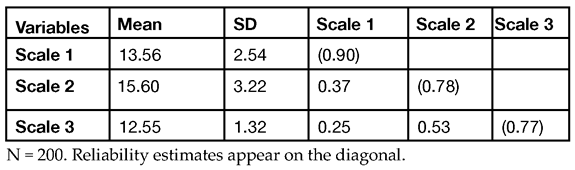
In Table 6.1, information for the first scale variable is in the intersection of the Scale 1 row and Scale 1 column. Where the row and column intersect, the coefficient alpha index for the first scale item is 0.90. Likewise, you see the coefficient alpha for Scale 2 where row 2 intersects with column 2 (alpha = 0.78), and the coefficient alpha for Scale 3 is where row 3 intersects with column 3 (alpha = 0.77).
When reliability estimates are computed for a relatively large number of scales, it is common to report them in a table (such as Table 6.1) and make only passing reference to them within the text of the paper when within acceptable parameters. For example, within a section on instrumentation, you might indicate the following:
“Estimates of internal consistency as measured by Cronbach’s alpha all exceeded 0.70 and are reported on the diagonal of Table 6.1.”
When reliability estimates are computed for only a small number of scales, it is possible to instead report these estimates within the body of the text itself. Here is an example of how this might be done:
“Internal consistency of scale responses was assessed by Cronbach’s alpha. Reliability estimates were 0.90, 0.78, and 0.77 for responses to Scale 1, Scale 2, and Scale 3, respectively.”
Summary
Assessing scale reliability with Cronbach’s alpha (or some other reliability index) should be one of the first tasks you undertake when conducting questionnaire research. If responses to selected scales are not reliable, there is no point in performing additional analyses. You can often improve suboptimal reliability estimates by deleting items with poor item-total correlations in keeping with the procedures discussed in this chapter. When several subscales on a questionnaire display poor reliability, it may be advisable to perform a principal component analysis or an exploratory factor analysis on responses to all questionnaire items to determine which tend to group together empirically. If many items load on
each retained factor and if the factor pattern obtained from such an analysis displays a simple structure, chances are good that responses to the resulting scales will demonstrate adequate internal consistency.
References
Clark, L. A., and Watson, D. 1995. “Constructing Validity: Basic Issues in Objective Scale Development.” Psychological Assessment, 7, 309–319.
Cortina, J. M. 1993. “What Is Coefficient Alpha? An Examination of Theory and Applications.” Journal of Applied Psychology, 78, 98–104.
Cronbach, L. J. 1951. “Coefficient Alpha and the Internal Structure of Tests.” Psychometrika, 16, 297–334.
DeVellis, R. F. 1991. Scale Development: Theory and Applications. Newbury Park, CA: Sage.
Henson, R. K. 2001.“Understanding Internal Consistency Estimates: A Conceptual Primer on Coefficient Alpha.” Measurement and Evaluation in Counseling and Development, 34, 177–189.
Nunnally, J. 1978. Psychometric Theory. New York: McGraw-Hill.
Spector, P. E. 1992. Summated Rating Scale Construction: An Introduction. Newbury Park, CA: Sage.