
 10
10
Multivariate Analysis of Variance (MANOVA) with One Between-Subjects Factor
Overview
This chapter shows how to use the Fit Model platform in JMP to perform a one-way multivariate analysis of variance (MANOVA). You can think of MANOVA as an extension of ANOVA that allows for the inclusion of multiple response variables in a single test. This chapter focuses on the between-subjects design, in which each subject is exposed to only one condition under the independent predictor variable. Examples show how to summarize both significant and nonsignificant MANOVA results.
Introduction: The Basics of Multivariate Analysis of Variance (MANOVA)
A Multivariate Measure of Association
Overview: Performing a MANOVAwith the Fit Model Platform
Example with Significant Differences between Experimental Conditions
Testing for Significant Effects with the Fit Model Platform
Steps to Interpret the Results
Formal Description of Results for a Paper?
Example with Nonsignificant Differences between Experimental Conditions
Summarizing the Results of the Analysis
Formal Description of Results for a Paper
Appendix: Assumptions Underlying MANOVA with One Between-Subjects Factor
Introduction: The Basics of Multivariate Analysis of Variance (MANOVA)
Multivariate analysis of variance (MANOVA) with one between-subjects factor is appropriate when the analysis involves
- a single nominal or ordinal predictor variable that defines groups
- multiple numeric continuous response variables
MANOVA is similar to ANOVA in that it tests for significant differences between two or more groups of participants. The important difference between MANOVA and ANOVA is that ANOVA is appropriate when the study involves just one response variable, but MANOVA is needed when there is more than one response variable. With MANOVA, you can perform a single test that determines whether there is a significant difference between treatment groups when compared simultaneously on all response variables.
To illustrate one possible use of MANOVA, consider the hypothetical study on aggression described in Chapter 8, “One-Way ANOVA with One Between-Subjects Factor.” In that study, each of 60 children is assigned to one of the following treatment groups based on consumption of sugar at lunch:
- 0 grams
- 20 grams
- 40 grams
A pair of observers watched each child after lunch, and recorded the number of aggressive acts displayed by that child. The total number of aggressive acts performed by a given child over a two-week period served as that child’s score on the aggression dependent variable. It is appropriate to analyze data from the aggression study with ANOVA because there is a single dependent variable—level of aggression.
Now consider how the study could be modified so that it is appropriate to analyze the data using a multivariate procedure, MANOVA. Imagine that, as the researcher, you want to have more than one measure of aggression. After reviewing the literature, you believe that there are at least four different types of aggression that children display:
- aggressive acts toward children of the same sex
- aggressive acts toward children of the opposite sex
- aggressive acts toward teachers
- aggressive acts toward parents
Assume that you want to replicate the earlier study, but this time the observers note the number of times each child displays an aggressive act in each of the four preceding categories. At the end of the two-week period, you have scores for each child on each of the categories. These four scores constitute four dependent variables.
You now have a number of options as to how you can analyze your data. One option is to perform four ANOVAs, as described in Chapter 8. In each ANOVA the independent variable is ”amount of sugar consumed.“ In the first ANOVA, the dependent variable is “number of aggressive acts directed at children of the same sex,” in the second ANOVA, the dependent variable is “number of aggressive acts directed at children of the opposite sex,” and so forth.
However, a better alternative is to perform a single test that assesses the effect of the independent variable on all four of the dependent variables simultaneously. This is what MANOVA can do. Performing a MANOVA allows you to test the following null hypothesis:
“In the population, there is no difference between the various treatment groups when they are compared simultaneously on the dependent variables.”
Here is another way of stating this null hypothesis:
“In the population, all treatment groups are equal on all dependent variables.”
MANOVA produces a single F statistic that tests this null hypothesis. If the null hypothesis is rejected, it means that at least two of the treatment groups are significantly different with respect to at least one of the dependent variables. You can then perform follow-up tests to identify the pairs of groups that are significantly different, and the specific dependent variables on which they are different. In doing these follow-up tests, you might find that the groups differ on some dependent variables (such as “aggressive acts directed toward children of the same sex”) but not on another dependent variables (such as “aggressive acts directed toward teachers”).
A Multivariate Measure of Association
Chapter 8 introduced the R2 statistic, which is a measure of association often computed by an analysis of variance. Values of R2 range from 0 to 1where higher values indicate a stronger relationship between the predictor variable and the response variable in the study. If the study is a designed experiment, you can view R2 as an index of the magnitude of the treatment effect.
This chapter introduces a multivariate measure of association that can be used when there are multiple response variables (as in MANOVA). This multivariate measure of association is called Wilks’ lambda. Values of Wilks’ lambda range from 0 to 1, but the way you interpret lambda is the opposite of the way that you interpret R2. With lambda, small values (near 0) indicate a relatively strong relationship between the predictor variable and the multiple response variables taken as a group, while larger values (near 1) indicate a relatively weak relationship. The F statistic that tests the significance of the relationship between the predictor and the multiple response variables is based on Wilks’ lambda.
The Commitment Study
To illustrate multivariate analysis of variance (MANOVA), assume you replicate the study that examined the effect of rewards on commitment in romantic relationships. However, this time modify the study to obtain scores on three dependent variables instead of just one.
It was hypothesized that the rewards people experience in romantic relationships have a causal effect on their commitment to those relationships. The one-way ANOVA analysis in Chapter 8 tested this hypothesis by conducting a type of role-playing experiment. All 18 participants in the experiment were asked to engage in similar tasks in which they read the descriptions of 10 potential romantic “partners.” For each partner, the participants imagined what it would be like to date this person, and rated how committed they would be to a relationship with that person. For the first 9 partners, every subject saw exactly the same description. However, the different experimental groups saw a slightly different description for partner 10.
For example, the 6 participants in the high-reward condition saw the following final sentence describe partner 10:
“This person enjoys the same recreational activities that you enjoy, and is said to be very good-looking.”
For the 6 participants in the mixed-reward condition, the last part of the description of partner 10 was worded:
“Sometimes this person seems to enjoy the same recreational activities that you enjoy, and sometimes not. Some people think partner 10 is very good looking, but others think not.”
For the 6 participants in the low-reward condition, the last sentence in the description of partner 10 read this way:
“This person does not enjoy the same recreational activities that you enjoy, and is not considered by most people to be very good-looking.”
In your current replication of the study from Chapter 8, you manipulate this “type of rewards” independent variable in exactly the same way. The only difference between the present study and the one described earlier involves the number of dependent variables obtained. In the earlier study, there was only one response variable, called Commitment. Commitment was defined as the participants’ rating of their commitment to remain in the relationship. Scores on this variable were created by summing participant responses to four questionnaire items.
However, in the present study you intend to obtain two additional dependent variables:
- participants’ ratings of their satisfaction with their relationship with partner 10
- participants’ rating of how long they intend to stay in the relationship with partner 10
Here, satisfaction is defined as the participants’ emotional reaction to partner 10, and the intention to stay is defined as the participants’ rating of how long they intend to maintain the relationship with partner 10. Assume that satisfaction and intention to stay in the relationship are measured with multiple items from a questionnaire, similar to those used previously to assess commitment.
You can see that there will be four values for each subject in the study. One value is for the classification variable that indicates whether the subject is assigned to the high-reward group, the mixed-reward group, or the low-reward group. The remaining three scores are the subject’s scores on the measures of commitment, satisfaction, and intention to stay in the relationship. In conducting the MANOVA, you want to determine whether there is a significant relationship between the type of rewards predictor variable and the three response variables taken as a group.
Overview: Performing a MANOVA with the Fit Model Platform
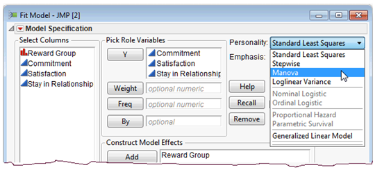
To do a multivariate analysis of variance in JMP, use the Fit Model command on the Analyze menu. The Fit Model dialog accepts multiple response variables when you specify the model. When there are multiple Y (response) variables, the personality types available are restricted to Standard Least Squares and Manova. The personality type specified for an analysis tells the Fit Model platform what kind of analysis to do.
When there are multiple Y variables, the default personality is Standard Least Squares, which does a univariate ANOVA for each response (four separate ANOVAs). In this context, univariate means one response variable. Each univariate ANOVA is the same analysis described in Chapter 8. The Standard Least Squares personality produces a univariate analysis of variance for the Commitment response, a second ANOVA for the Satisfaction response, and a third analysis for the variable called Stay in Relationship. This chapter introduces the Manova personality.
Figure 10.1 shows an example of the Fit Model dialog with multiple Y variables, and the available personality types. The Manova personality does the multivariate analysis of variance described in the next sections of this chapter. In the example, you complete the dialog and select the Manova personality, as shown here.
In the context of a MANOVA, multivariate means multiple response variables. For your purposes, these multivariate results consist of Wilks’ lambda and the F statistic derived from Wilks’ lambda.
Figure 10.1: Fit Model Platform with Multiple Responses
There is a specific sequence of steps to follow when interpreting these results.
Step 1: First, review the multivariate F statistic derived from Wilks’ lambda. If this multivariate F statistic is significant, you can reject the null hypothesis of no overall effect for the predictor variable. In other words, you reject the null hypothesis that, in the population, all groups are equal on all response variables. At that point, you perform and interpret a univariate ANOVA for each response.
Step 2: To interpret the ANOVAs, first identify those response variables for which the univariate F statistic is significant. If the F statistic is significant for a given response variable, then go on to interpret the results of the Tukey’s HSD (Honestly Significant Difference) multiple comparison test to determine which pairs of groups are significantly different from one another.
Step 3: However, if the multivariate F statistic that is computed in the MANOVA is not significant, you cannot reject the null hypothesis that all groups have equal means on the response variables in the population. In most cases, your analysis should terminate at that time. You don’t usually proceed with univariate ANOVAs.
Step 4: Similarly, even if the multivariate F statistic is significant, you should not interpret the results for any specific response variable that did not display a significant univariate F statistic. This is consistent with the general guidelines for univariate ANOVA presented in Chapter 8, “One-Way ANOVA with One Between-Subjects Factor.”
Example with Significant Differences between Experimental Conditions
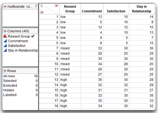
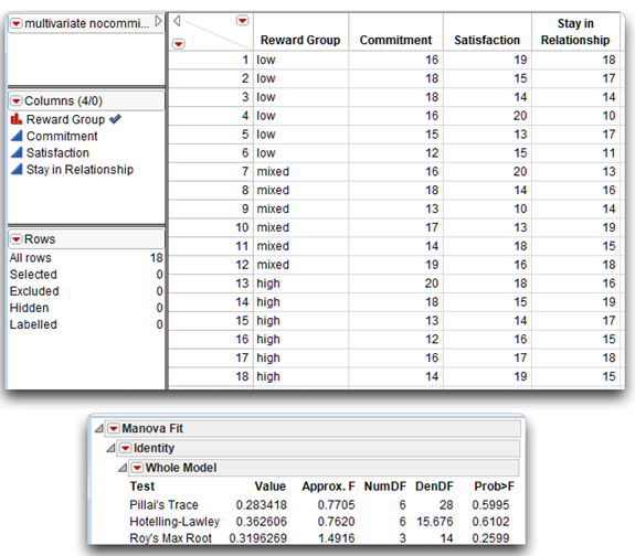
Assume the study is complete and the data are entered into a JMP table. The data table, multivariate commitment.jmp, is shown in Figure 10.2.
There is one predictor variable in this study called Reward Group. This variable can assume the values “low” to represent participants in the low-reward group, “mixed” for participants assigned to the mixed-reward group, or “high” for participants in the high-reward group.
There are three response variables in this study. The first response variable, Commitment, is a measure of the subject’s commitment to the relationship. The second response, Satisfaction, measures the subject’s satisfaction with the relationship, and the third response, called Stay in Relationship, measures the subject’s intention to stay in the relationship. Each variable has a possible score that ranges from a low of 4 to a high of 36.
Note: The check mark icon to the right of the Reward Group name in the Columns panel in the data table indicates it has the List Check column property, which lets you specify the order you want variable values to appear in analysis results. It also restricts the allowable values in the column to the ones you list. In this example, you want to see the Reward Group values listed in the order, “low,” “mixed,” and “high.” Unless otherwise specified, values in reports appear in alphabetic order. See the “Ordering Values in Analysis Results” section in Chapter 9, “Factorial ANOVA with Two Between-Subjects Factors,” for details about using the List Check property.
Figure 10.2: Multivariate Data for Commitment Study
Testing for Significant Effects with the Fit Model Platform
The following example shows a step-by-step example of how to use the Fit Model platform in JMP to perform a multivariate analysis of variance and explains the results.
![]() Open the table shown in Figure 10.2, called multivariate commitment.jmp, with one predictor variable, Reward Group, and three response variables, Commitment, Satisfaction, and Stay in Relationship.
Open the table shown in Figure 10.2, called multivariate commitment.jmp, with one predictor variable, Reward Group, and three response variables, Commitment, Satisfaction, and Stay in Relationship.
![]() Choose Fit Model from the Analyze menu.
Choose Fit Model from the Analyze menu.
![]() When the Fit Model dialog appears, complete the dialog as shown in Figure 10.1. Be sure you select Manova from the Personality menu.
When the Fit Model dialog appears, complete the dialog as shown in Figure 10.1. Be sure you select Manova from the Personality menu.
![]() Click Run to see the initial results, which are shown in Figure 10.3.
Click Run to see the initial results, which are shown in Figure 10.3.
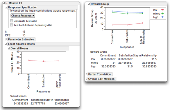
When you do a MANOVA, the results unfold as you provide additional information to the platform. To begin, you see the Response Specification panel on the left in Figure 10.3, which lets you specify the next step in the analysis. The initial results also include the overall means, group means, and means plots.
Initial Means and Plots
As with most JMP analyses, initial results show summary statistics and supporting plots or graphs whenever possible. For example, the first MANOVA results include a table of overall means for the response variables, and a plot of those means showing beneath the Response Specification panel. You can quickly see that the overall means don’t appear to vary across the responses. The next table and corresponding plots are the means for each response in the three levels of the predictor variable, Reward Group. The plot for these means indicates that responses for the high-reward group and the mixed-reward group are similar, but the levels for the low-reward group are much lower for each response.
Note that the Response Specification panel also shows the total observations in the sample, N, and the error degrees of freedom, DFE, for the analysis. These items give you a verification that data are what you intended—that the number of observations (N) in the data table is correct, and the number of predictor groups is N less the error degrees of freedom (18 – 15 = 3 groups).
Figure 10.3: Initial Results of MANOVA Analysis
The Response Specification Panel
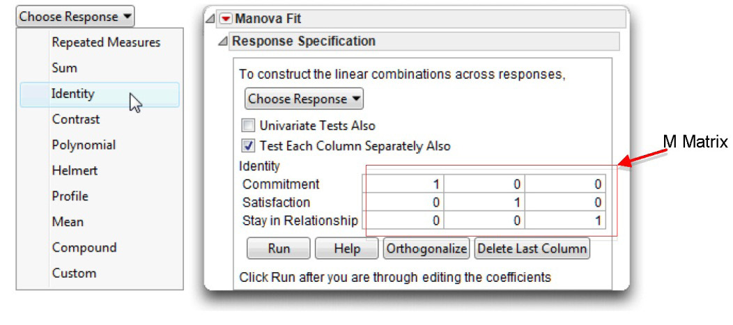
You use the Response Specification panel (top left in Figure 10.3) to specify the response design for the kind of multivariate tests you want to see. The menu on the left in Figure 10.4 shows the choices available for multivariate comparisons. The choice you make defines the M Matrix used in the analysis. The columns in the M matrix define a set of transformation variables used to compute the multivariate tests. It is easiest to understand the M matrix and corresponding multivariate tests by looking at the M matrix. To do this,
![]() Select different options from the Choose Response menu and look at the M matrix appended to the Response Specification panel by the choice you make.
Select different options from the Choose Response menu and look at the M matrix appended to the Response Specification panel by the choice you make.
One of the most commonly used response designs is Identity, which is used for this example. It is the standard design used to test the multivariate responses as a group. Descriptions and details for all the choices are in Modeling and Multivariate Methods (2012) available on the Help menu.
![]() Choose Identity from the Choose Response menu on the Response Specification panel.
Choose Identity from the Choose Response menu on the Response Specification panel.
![]() Click Run to see the MANOVA results.
Click Run to see the MANOVA results.
Figure 10.4: Response Specification Panel
Steps to Interpret the Results
You can state the multivariate null hypothesis for the present study as follows:
“In the population, there is no difference between the high-reward group, the mixed-reward group, and the low-reward group when they are compared simultaneously on commitment, satisfaction, and intention to stay in the relationship.”
In other words, in the population, the three groups are equal on all response variables. Symbolically, you can represent the null hypothesis this way:
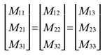
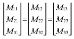
Each M represents a population mean for one of the treatment conditions on one of the response variables. The first number in each subscript identifies the response variable and the second number identifies the experimental group. Since the List Check option orders the Reward Group values as “low,” “mixed,” and “high,” M32 refers to the population mean for the third response variable (intention to stay in relationship) in the second experimental group (the mixed-reward group), while M13 refers to the population mean for the first response variable (commitment) in the third experimental group (the high-reward group).
Review Wilks’ Lambda, the Multivariate F Statistic, and Its p-Value
The F statistic appropriate to test this null hypothesis is in the Whole Model table of the Manova Fit results. Note in Figure 10.5 that because Reward Group is the only effect the results for the effect and the whole model are the same. This would not be the case if there were more effects. The Whole Model table provides the results from four different multivariate tests, but you want to focus only on Wilks’ lambda.
Figure 10.5: Results from Multivariate Analysis with Significant Results
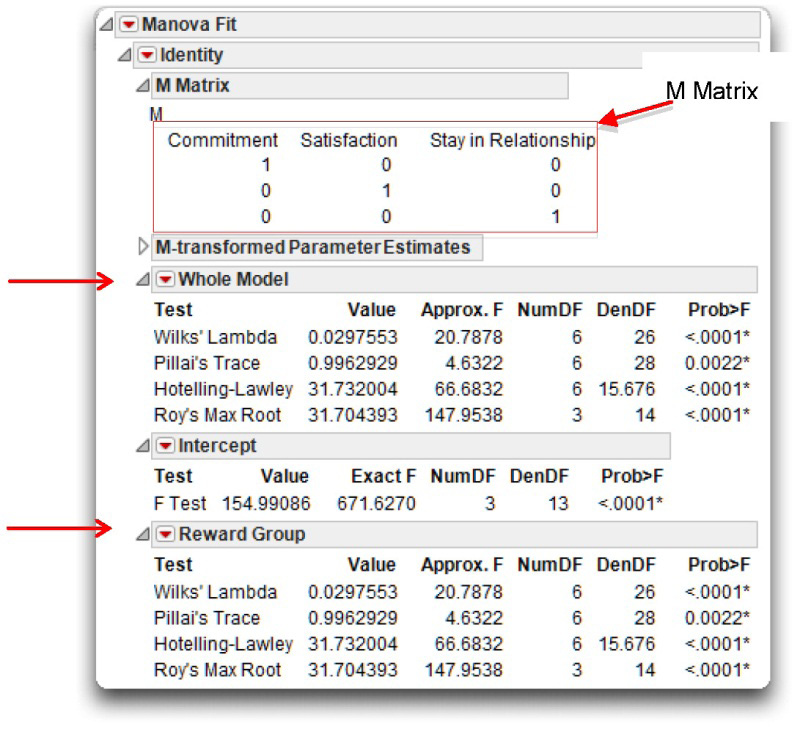
Information for Wilks’ lambda shows in the first line of the table. Read the information from this row only. Where the row heading Wilks’ Lambda intersects with the column heading Value, you find the computed value of the Wilks’ lambda statistic. For the current analysis, lambda is 0.0297553. Remember that small values (closer to 0) indicate a relatively strong relationship between the predictor variable and the multiple response variables, and so this obtained value (rounded to 0.03) indicates that there is a strong relationship between Reward Group and the response variables. This is an exceptionally low value for lambda, much lower than you are likely to encounter in actual research.
This value for Wilks’ lambda indicates that the relationship between the predictor and the response is strong, but to see if it is statistically significant, look at the multivariate F statistic, shown under the heading Approx. F. You can see that the multivariate F for this analysis is approximately 20.79. There are 6 numerator degrees of freedom and 26 denominator degrees of freedom associated with this test, as seen under the headings Num DF and Den DF. The probability value for this F appears under the heading Pr > F, showing that the
p-value is very small, less than 0.0001. Because this p-value is less than the standard cut off of 0.05, you can reject the null hypothesis of no differences between groups in the population. In other words, you conclude that there is a significant multivariate effect for type of rewards.
Univariate ANOVAs and Multiple Comparisons
When the MANOVA F test is significant, you might want to look at the univariate ANOVA and Tukey’s HSD test for each individual response. An easy way to do this is to use the Fit Model dialog as shown previously for the multivariate analysis, but change the personality to Standard Least Squares.
![]() Click the Fit Model dialog to make it the active window. Or, if you previously closed this dialog, select Fit Model from the Analyze menu again, and enter the same responses and factors as before (see Figure 10.1).
Click the Fit Model dialog to make it the active window. Or, if you previously closed this dialog, select Fit Model from the Analyze menu again, and enter the same responses and factors as before (see Figure 10.1).
![]() Use the default personality, Standard Least Squares, and change the emphasis to Minimal Report, as shown in Figure 10.6.
Use the default personality, Standard Least Squares, and change the emphasis to Minimal Report, as shown in Figure 10.6.
Figure 10.6: Personality and Emphasis in the Fit Model Dialog
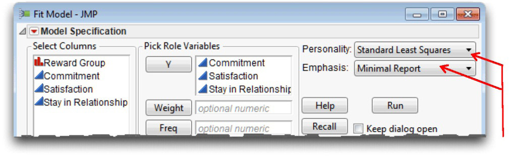
The Standard Least Squares personality (as opposed to Manova) performs an analysis of variance on each of the specified Y responses. The Minimal Report selection from the Emphasis menu suppresses some of the results, which is appropriate in this example because you are only interested in the univariate ANOVA and Tukey’s HSD tests.
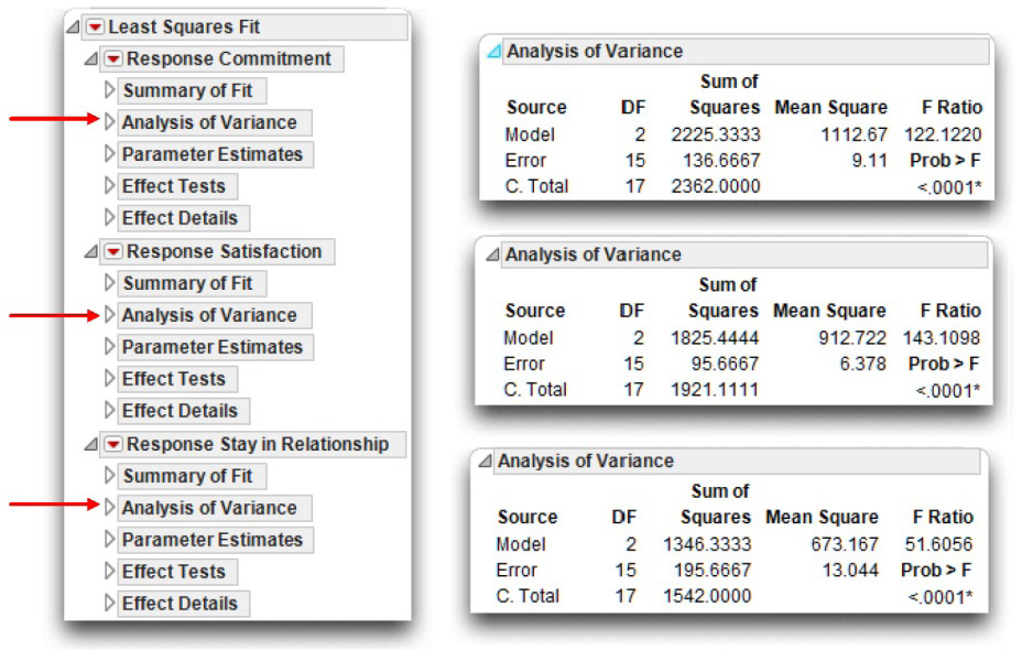
![]() Click Run to see the results. Because the only results of interest are the analysis of variance and Tukey HSD tests, first close all open reports, which then displays the outline nodes shown in the left in Figure 10.7.
Click Run to see the results. Because the only results of interest are the analysis of variance and Tukey HSD tests, first close all open reports, which then displays the outline nodes shown in the left in Figure 10.7.
![]() Open the Analysis of Variance reports for each response. The analysis of variance for each response variable shows on the right in Figure 10.7. All three responses have significant F tests with probabilities less than 0.0001, which means you want to look at Tukey’s HSD for each response.
Open the Analysis of Variance reports for each response. The analysis of variance for each response variable shows on the right in Figure 10.7. All three responses have significant F tests with probabilities less than 0.0001, which means you want to look at Tukey’s HSD for each response.
Figure 10.7: Univariate ANOVA for the Three Responses
![]() To see Tukey’s HSD multiple comparison tests, first open the Effect Details report for each of the three response variables. This report begins with the Least Squares means table, shown here. The Effect Details table shows the mean and standard error for each group level.
To see Tukey’s HSD multiple comparison tests, first open the Effect Details report for each of the three response variables. This report begins with the Least Squares means table, shown here. The Effect Details table shows the mean and standard error for each group level.
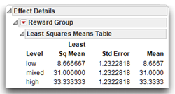
Note: The LSMeans (Least Squares Means) and the Mean are the same when there are no interaction terms in the model. However, they can be different for a main effect when the design is unbalanced (group sample sizes are different).
![]() Each response shows the Reward Group effect. Select LSMeans Tukey HSD from the menu on the Reward Group title bar for each response.
Each response shows the Reward Group effect. Select LSMeans Tukey HSD from the menu on the Reward Group title bar for each response.
Figure 10.8: Tukey’s HSD Multiple Comparison Tests for Commitment Response
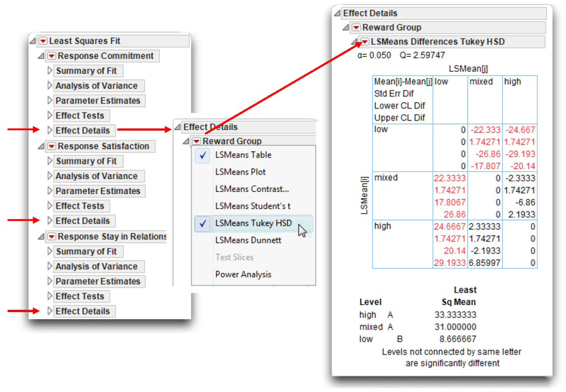
The alpha level of 0.05 is at the top of the report. The multiple comparisons statistical results in Figure 10.8 show as a crosstabs table followed by the letter report.
- The crosstabs report is a two-way table that gives the difference in the group means, standard error of the difference, and confidence levels. Significant differences are highlighted (in red).
- The letter report is a quick way to see differences. Groups (levels) connected by the same letter are not significantly different. The Tukey HSD tests confirm the graphical results seen previously in Figure 10.3. For each of the responses, the high-reward and mixed-reward groups are not statistically different from each other, but both are different from the low-reward group.
Summarize the Results of the Analysis
This section shows how to summarize the results of the multivariate test discussed in the previous section. When the multivariate test is significant, proceed to the univariate ANOVAs and summarize them using the format presented in Chapter 8. To see multiple comparisons between group levels, do a univariate ANOVA for each response and look at Tukey’s HSD, as described in the previous section.
You can use the following statistical interpretation format, similar to previously shown formats, to summarize the multivariate results from a MANOVA:
A. Statement of the problem
B. Nature of the variables
C. Statistical test
D. Null hypothesis (Ho)
E. Alternative hypothesis (H1)
F. Obtained statistic
G. Obtained probability (p) value
H. Conclusion regarding the multivariate null hypothesis
I. If the MANOVA p-value is significant, perform ANOVA on each response
J. For responses with significant ANOVA results, look at Tukey’s HSD multiple comparisons
K. Conclusion regarding group differences for individual responses
You could summarize the preceding MANOVA analysis in this way:
A. Statement of the problem
The purpose of this study was to determine whether there was a difference between people in a low-reward relationship, people in a mixed-reward relationship, and people in a high-reward relationship with respect to their commitment to the relationship, their satisfaction with the relationship, and their intention to stay in the relationship.
B. Nature of the variables
This analysis involved one predictor variable and three response variables. The predictor variable was type of rewards, a nominal variable that could assume three values—low-reward, mixed-reward, and a high-reward. The three continuous numeric response variables were commitment, satisfaction, and intention to stay in the relationship.
C. Statistical test
Wilks’ lambda, derived through a one-way MANOVA between-subjects design.
D. Null hypothesis (H0)
“In the population, there is no difference between people in a low-reward relationship, people in a mixed-reward relationship, and people in a high-reward relationship when they are compared simultaneously on commitment, satisfaction, and intention to stay in the relationship.”
E. Alternative hypothesis (H1)
In the population, there is a difference between people in at least two of the conditions (low-reward, mixed-reward, and high-reward conditions), when they are compared simultaneously on commitment, satisfaction, and intention to stay.
F. Obtained statistic
Wilks’ lambda = 0.03, with corresponding F (6, 26) = 20.79.
G. Obtained probability (p) value
p < 0.0001.
H. Conclusion regarding the null hypothesis
Reject the multivariate null hypothesis.
I. Perform ANOVA on each response variable
Difference between groups was significant for all response variables
p< 0.0001.
J. Multiple comparison results
For each response, Tukey’s HSD multiple comparisons showed that the high-reward and mixed-reward groups were not statistically different from each other but both were different from the low-reward group.
Formal Description of Results for a Paper
You could summarize this analysis in the following way for a professional journal:
Results were analyzed using one-way MANOVA between-subjects design. This analysis revealed a significant multivariate effect for type of rewards, Wilks’ lambda = .03, F(6, 26) = 20.79; p < 0.0001. Subsequent univariate ANOVA of the response variables showed significant differences between groups for each response. For each response, Tukey’s HSD multiple comparisons showed that the high-reward and mixed-reward groups were not statistically different from each other but both were different from the low-reward group.
Example with Nonsignificant Differences between Experimental Conditions
To continue, perform MANOVA a second time, but this time use the data table called multivariate nocommitment.jmp. This table is constructed to provide nonsignificant results. Proceed with a multivariate analysis as shown in the previous section. Use Fit Model in the Analyze menu. On the Fit Model dialog,
![]() Select Commitment, Satisfaction, and Stay in Relationship, in the Select Column lists, and then click Y.
Select Commitment, Satisfaction, and Stay in Relationship, in the Select Column lists, and then click Y.
![]() Select Reward Group, and then click Add.
Select Reward Group, and then click Add.
![]() Select Manova from the Personality menu.
Select Manova from the Personality menu.
![]() Click Run to see the results.
Click Run to see the results.
The results are shown beneath the data table in Figure 10.9. This analysis computed a value for Wilks’ lambda of 0.726563. Because this is a relatively large number (closer to 1), it indicates that the relationship between type of rewards and the three response variables is weaker with this data set than with the previous data set.
This analysis produced a multivariate F of only 0.75, which, with 6 and 26 degrees of freedom, is nonsignificant (p = 0.615). Therefore, this analysis fails to reject the multivariate null hypothesis of no group differences in the population. Because the multivariate F is not significant, your analysis usually terminates at this point—you would not go on to interpret univariate ANOVAs for the responses.
Figure 10.9: Data and Multivariate Analysis with No Significant Results
Summarizing the Results of the Analysis
Because this analysis tested the same null hypothesis that you tested earlier, you would prepare items A through E in the same manner described before. Therefore, this section presents only items F through H of the statistical interpretation format:
F. Obtained statistic
Wilks’ lambda = 0.73, corresponding F = 0.75.
G. Obtained probability (p-value)
p = 0.615.
H. Conclusion regarding the multivariate null hypothesis
Fail to reject the null hypothesis.
Formal Description of Results for a Paper
Results were analyzed using one-way MANOVA between-subjects design. This analysis failed to reveal a significant multivariate effect for type of rewards, Wilks’ lambda = 0.73, F(6, 26) = 0.75; p = 0.615.
Summary
Chapters 8, 9, and 10 of this book focused on between-subject research designs—designs in which each subject is assigned to just one treatment condition, and provide data only under that condition. However, in some situations it is advantageous to conduct studies in which each subject provides data under every treatment condition. This type of design is called a repeated-measures design, and requires data analysis techniques that differ from the ones presented in the last three chapters. The next chapter introduces procedures for analyzing data from the simplest type of repeated-measures design.
Appendix: Assumptions Underlying MANOVA with One Between-Subjects Factor
Level of measurement, data type, and modeling type
Each response variable should be a continuous numeric variable (an interval-level or ratio-level of measurement). The predictor variable should be a categorical (nominal-level) variable (a categorical variable).
Independent observations
Across participants, a given observation should not be dependent on any other observation in any group. It is acceptable for the various response variables to be correlated with one another. However, a given subject’s score on any response variable should not be affected by any other subject’s score on any response variable. For a more detailed explanation of this assumption, see Chapter 7, “t-Tests: Independent Samples and Paired Samples.”
Random sampling
Scores on the response variables should represent a random sample drawn from the populations of interest.
Multivariate normality
In each group, scores on the various response variables should follow a multivariate normal distribution. Under conditions normally encountered in social science research, violations of this assumption have only a very small effect on the type I error rate (the probability of incorrectly rejecting a true null hypothesis). On the other hand, when the data are platykurtic (form a relatively flat distribution), the power of the test may be significantly attenuated. The power of the test is the probability of correctly rejecting a false null hypothesis. Platykurtic distributions may be transformed to better approximate normality (see Stevens, 2002, or Tabachnick and Fidell, 2001).
Homogeneity of covariance matrices
In the population, the response-variable covariance matrix for a given group should be equal to the covariance matrix for each of the remaining groups. This is the multivariate extension of the homogeneity of variance assumption in univariate ANOVA.
To illustrate, consider a simple example with two groups and three response variables (V1, V2, and V3). To satisfy the homogeneity assumptions, the variance of V1 in group 1 must equal (in the population) the variance of V1 in group 2. The same must be true for the variances of V2 and V3. In addition, the covariance between V1 and V2 in group 1 must equal (in the population) to the covariance between V1 and V2 in group 2. The same must be true for the remaining covariances (between V1 and V3 and between V2 and V3).
It becomes clear that the number of corresponding elements that must be equal increases dramatically as the number of groups increases and/or as the number of response variables increases. For this reason, the homogeneity of covariance assumption is rarely satisfied in real-world research. Fortunately, the Type I error rate associated with MANOVA is relatively robust against typical violations of this assumption so long as the sample sizes are equal. However, the power of the test tends to be attenuated when the homogeneity assumption is violated.
References
SAS Institute Inc. 2003. JMP Statistics and Graphics Guide. Cary, NC: SAS Institute Inc.
Stevens, J. 2002. Applied Multivariate Statistics for the Social Sciences, Fourth Edition. Mahwah, NJ: Lawrence Erlbaum Associates.
Tabachnick, B. G., and Fidell, L. S. 2001. Using Multivariate Statistics, Fourth Edition. New York: Harper Collins.