
Chapter 10. Java Enterprise Edition Performance
This chapter focuses on using JavaEE—specifically, JavaEE 6 and 7. It covers JSPs, servlets, and EJB 3.0 Session Beans—though not EJB 3.0 Entity Beans (Java Persistence API entities), since the are not specifically a JavaEE technology (they are discussed in depth in Chapter 11).
Basic Web Container Performance
The heart of a JavaEE application server is the performance of its web container, which handles HTTP requests via basic servlets and JSP pages.
Here are the basic ways to improve performance of the web container. The details of how these changes are made vary depending on the Java EE implementation, but the concepts apply to any server.
Produce less output
Producing less output will speed up the time it takes your web page to get to the browser.
Produce less whitespace
In servlet code, don’t put whitespace in calls to the
PrintWriter; that whitespace takes time to transmit over the network (and, for that matter, to process in the code, but the network time is more important). This means you should call theprint()method in preference to theprintln()method, but it primarily means not writing tabs or spaces to reflect the structure of the HTML. It is true that someone who views the source of the web page won’t see its structure, though they can always use an XML or HTML editor if they’re really interested in that. That applies to an in-house QA or performance group too: certainly it makes my job easier when debugging a web page if the source reflects the structure of the page. But in the end, I’ll put up with loading the source into a formatting editor in order to improve the application’s response time.Most application servers can trim the whitespace out of JSPs automatically; e.g., in Tomcat (and open-source Java EE servers based on Tomcat), there is a
trimSpacesdirective that will trim out any leading and trailing white space from JSP pages. That allows the JSP pages to be developed and maintained with correct (for humans, at least) indentation, but not pay the penalty for transmitting all that needless whitespace over the network.Combine CSS and JavaScript resources
As a developer, it makes sense to keep CSS resources in separate files; they are easier to maintain that way. The same is true of JavaScript routines. But when it comes time to serve up those resources, it is much more efficient to send one larger file rather than a several smaller files.
There is no JavaEE standard for this, nor a way to do it automatically in most application servers. But there are several development tools that can help you combine those resources.
Compress the output
From the perspective of the user sitting at her browser, the longest time in executing a web request is often the time required to send the HTML back from the server. This is something that is frequently missed in performance testing, since performance testing between clients (emulating browsers) and servers often occurs over fast, local-area networks. Your actual users might be on a “fast” broadband network, but that network is still an order of magnitude slower than the LAN between the machines in your lab.
Most application servers have a mechanism to compress the data sent to the browser: the HTML data is compressed and sent to the browser with a content-type of
ziporgzip. This is done only if the original request indicates that the browser supports compression. All modern browsers support that feature.Enabling compression requires more CPU cycles on the server, but the smaller amount of data usually takes less time to traverse the network, yielding a net improvement. However, unlike the other optimizations discussed in this section, it is not universally an improvement; examples later in this section show that when compression is enabled on a LAN, performance may decrease. The same is true for an applications that sends very small pages (though most application servers will allow output to be compressed only if it is larger than some specified size).
Don’t use dynamic JSP compilation
By default, most Java EE application servers will allow a JSP page to be changed on the fly: the JSP file can be edited in place (wherever it is deployed), and those changes will be reflected the next time the page is visited. That’s quite useful when a new JSP is being developed, but in production it slows down the server, since every time the JSP is accessed, the server must check the last modified date on its file to see if the JSP needs to be reloaded.
This tunable is often called development mode, and it should be off in production and for performance testing.
These optimizations can make a significant difference in real-world (as opposed to laboratory) performance. Table 10-1 shows the kind of results that might be expected. Tests were run using the long-output form of the stock history servlet, retrieving data for a 10-year period. This results in an uncompressed, untrimmed HTML page of about 100 KB. To minimize the effect of bandwidth considerations, the test ran only a single user with a 100 millisecond think time and measured the average response time for requests. In the LAN case, tests were run over a local network with a 100 MB switch connecting components; in the Broadband case, tests were run over my home machine’s cable modem (where I average 30 mbits/second download speed). The WAN case uses the public WiFi connection in my local coffee shop—the speed of which is fairly unreliable (the table shows the average of samples over a 4-hour period).
| Optimization Applied | ART on LAN | ART on Broadband | ART on Public Wifi |
None | 20 ms | 26 ms | 1003 ms |
Whitespace removed | 20 ms | 10 ms | 43 ms |
Output Compressed | 30 ms | 5 ms | 17 ms |
This highlights is the importance of testing in the environment where the application will actually be deployed. If only the lab test were used to inform tuning choices, 80% of performance would have been left on the table. Although the non-laboratory tests in this case were run to a remote application server (utilizing a public cloud service), there are hardware-based emulators that can simulate such connectivity in a lab environment, hence allowing control over all the machines involved.
Quick Summary
- Test Java EE applications on the network infrastructure(s) where they will actually be tested.
- External networks are still relatively slow. Limiting the amount of data an application writes will be a big performance win.
HTTP Session State
There are two important performance tips regarding HTTP session state.
HTTP Session State Memory
Pay attention to the way in which HTTP session state is managed in an application. HTTP session data is usually long-lived, so it is quite easy to fill the heap up with session state data. That leads to the usual issues when GC needs to run too frequently.[58]
This is best dealt with at an application level: think carefully before deciding to store something in the HTTP session. If the data can be easily recreated, it is probably best left out of the session state. Also be aware of how long the session state is kept around. This value is stored in the web.xml file for an application and defaults to 30 minutes:
<session-timeout>30</session-timeout>
That’s a long time to keep session data around—is a user really expected to return after a 29-minute absence? Reducing that value can definitely mitigate the heap impact of having too much session data.
This is an area where the implementation of the Java EE application server can help. Although the session data must be available for 30 minutes (or whatever value is specified), the data doesn’t necessarily have to remain in the Java heap. The application server can move the session data (by serializing it) to disk or a remote cache—say, maybe after 10 minutes of idle time. That frees up space within the application server’s heap and still fulfills the contract with the application to save the state for 30 minutes. If the user does come back after 29 minutes, her first request might take a little longer as the state is read back from disk, but overall performance of the application server will have been better in the meantime.
This is also an important principle to keep in mind while testing: what is the realistic expectation for session management among the users of the application? Do they log in once in the morning and use that session all day? Do they come and go frequently, leaving lots of abandoned sessions on the server? Something in-between? Whatever the answer is, make sure that testing scenario reflects the expected use of the session. Otherwise, the production server will be ill-tuned, since its heap will be utilized in a completely different way than the performance tests measured.
Load generators have different ways of managing sessions, but in general
there will be an option to start a new session at certain points of the
testing (which is accomplished by closing the socket connection to the
server and discarding all previous cookies). In the tests throughout this
book using
fhb, a single session is maintained throughout each test for each
client thread.[59]
Highly-Available HTTP Session State
If an application server is tested in a highly-available (HA) configuration, then you must also pay attention to how the server replicates the session state data. The application server has the choice to replicate the entire session state on every request, or to replicate only the data that has changed. It should come as no surprise that the second option is almost always the more performant solution. Once again, this is a feature that is supported by most application servers but that is set in a vendor-specific way. Consult the appserver documentation regarding how to replicate on an attribute basis.
However, for this solution to
work, developers must follow guidelines about how session state is handled.
In
particular, the application server cannot keep track of changes to
objects that are already
stored in the session. If an object is retrieved from a session and then
changed, the
setAttribute()
method must be called to let the application server know that the value of
the object has changed:
HttpSessionsession=request.getSession(true);ArrayList<StockPriceHistory>al=(ArrayList<StockPriceHistory>)session.getAttribute("saveHistory");al.add(...somedata...);session.setAttribute("saveHistory",al);
That final call to
setAttribute()
is not required in a single (non-replicated) server:
the array list is already in the session state. If that call is omitted and
all future requests for this session return to this server,
everything will work correctly.
If that call is omitted, the session is replicated to a backup server, and
a request is then processed by the backup server, the application may find that
the data in the array list has not been changed. This is because the
application server “optimized” its session state handling by only copying
changed data to the backup server. Absent a call to the
setAttribute()
method, the application server had no idea that the array list was changed,
and so did not replicate it again after the above code was executed.
This is a somewhat murky area of the Java EE specification. The spec does not
mandate that the
setAttribute()setAttribute()
method would
still function correctly. That works functionally, but the performance will be
much worse than if the appserver could replicate only the changed attributes.
The moral of the story: call the
setAttribute()
method whenever you change
the value of an object stored in the session state, and make sure that
your application server is configured to replicate only changed data.
Quick Summary
- Session state can have a major impact on the performance of an application server.
- To reduce the effect of session state on the garbage collector, keep as little data in the session state as possible, and expire the session as soon as possible.
- Look into appserver-specific tunings to move stale session data out of the heap.
- When using high availability, make sure to configure the application server only to replicate attributes that have changed.
Thread Pools
Thread pools are covered in depth in Chapter 9. Java EE servers make extensive use of such pools; everything that chapter says about properly sizing the thread pool applies to application servers.
Application servers typically have more than one thread pool. One thread pool is commonly used to handle servlet requests; another handles remote EJB requests; a third might handle JMS requests. Some application servers also allow multiple pools to be used for for each kind of traffic: e.g., servlet requests to different URLs—or calls to different remote EJBS—can be handled by separate thread pools.
Separate thread pools allow a limited prioritization of different traffic within the application server. Take the case of an application server that is running on a machine with four CPUs; assume that its HTTP thread pool has 12 threads and its EJB thread pool has four. All threads will compete for the CPU, but when all threads are busy, a servlet request will be three times more likely than an EJB request to get access to the CPU. In effect, the servlet is given a 3x priority.
There are limitations to this. The separate pools cannot be set so that an EJB request would run only if there were no servlet requests that are pending. As long as there are threads in the EJB thread pool, those threads will compete equally for the CPU, no matter how busy the servlet thread pool is.
Similarly, care should be taken not to throttle a particular pool below the amount of work expected when the server is otherwise idle. If the JMS pool is sized to have only three threads on the four CPU machine, then it won’t use all of the available CPU if there are only JMS requests to process. To compensate for that, the size of all pools can be increased proportionally, but then you run the risk of over-saturating the machine by trying to run too many threads.
Hence, this kind of tuning is quite delicate and depends on having a good model of the traffic into your application server. It is used to get that last few percentage points of performance from your application.
Enterprise Java Session Beans
This section looks into the performance of EJB 3.0 session beans. Java EE containers manage the lifecycle of an EJB in a very specific way; the guidelines in this section can help make sure that that lifecycle management doesn’t impact the application’s performance.
Tuning EJB pools
EJBs are stored in object pools because they can be quite expensive to construct (and destroy). Without pooling, a call to an EJB would involve these steps:
- Create the EJB object
- Process annotations and inject any resource dependencies into the new EJB
-
Call any method annotated with
@PostConstruct -
For stateful beans, call any method annotated with
@Init, or call theejbCreate()method - Execute the business method
-
Call any method annotated with
@PreRemove -
For stateful beans, call the
remove()method
When the EJB is obtained from a pool, only the business method needs to be executed—the other six steps can be skipped. Though object pooling is not necessarily useful in the general case (see Chapter 7), this is one case where the expense of initializing an object makes pooling worthwhile.
This performance benefit only accrues if there is an available EJB object in the application server’s pool—so the application server must be tuned to support the expected number of EJBs an application will simultaneously use. If an application uses an EJB and there are no pooled instances, the application server will go through the entire lifecycle of creating, initializing, using, and destroying the EJB object.
The number of objects an application needs depends, of course, on how the application is used. A typical starting point is to make sure that there are as many objects in the EJB pool as there are worker threads in the application server, since it is common that each request will need at most one EJB. Note that EJB pools are per type: if an application has two EJB classes, the application server will use two pools (each of which can be sized to the number of threads in the pool).
Application servers differ in the way EJB pools are tuned, but the common case is that there is a global (or default) configuration for each EJB pool, and individual EJBs that need a different configuration can override that (often in their deployment descriptors). For instance, in the GlassFish application server, the EJB container uses a default of 32 EJB instances in each pool, and set the size of an individual bean’s pool can be set with this stanza it the sun-ejb-jar.xml file:
<bean-pool>
  <steady-pool-size>8</steady-pool-size>
  <resize-quantity>2</resize-quantity>
  <max-pool-size>64</max-pool-size>
  <pool-idle-timeout-in-seconds>300</pool-idle-timeout-in-seconds>
</bean-pool>
This doubles the maximum size of the bean’s EJB pool to 64.
The penalty for creating an EJB pool size that is too big is not usually very large. Unused instances in the pool will mean that GC will be slightly less efficient, but the pool sizes in general should be so small that the unused instances don’t have a significant impact. The exception is if the bean holds onto a lot of memory, in which case the GC penalty starts to grow. However, as can be deduced from the above XML stanza, the common way for an application server to manage the pool is to have a steady size in addition to a maximum size. In the example above, if traffic comes in such that at most 10 instances of this EJB (e.g., from 10 simultaneous requests) are used, only 10 EJB instances will ever be created—the pool will never begin to approach its maximum of 64.
If there is a brief traffic spike, the pool might create those 64 instances, but as the traffic wanes, those additional EJBs will be idle. Once they are idle for 300 seconds, they will be destroyed and their memory eligible for GC. This minimizes the effect of the pool on GC.
Hence, be more concerned about tuning the steady size of EJB pools than the maximum size.
Quick Summary
- EJB pools are a classic example of object pooling: they are effectively pooled because they can be expensive to initialize, and because there are relatively few of them.
- EJB pools generally have a steady and maximum size. Both values should be tuned for a particular environment, but the steady size is more important to minimize long-term effects on the garbage collector.
Tuning EJB Caches
There is another consideration for stateful session beans, which is that they are subject to passivation: in order to save memory, the application server can choose to serialize the state of the bean and save it to disk. This is a severe performance penalty and in most cases is best avoided.
Just how do you know what values to use for the size of the EJB pools and caches? One way is to make an educated guess based on knowledge of how the application works in conjunction with its expected load. But the only way actually to know if too many EJBs are being created (or too many stateful session beans are being passivated) is to use the monitoring facilities of the application server.
Figure 10-1 shows an example of how the monitoring is accomplished in GlassFish. In this case, the number of EJBs destroyed is not zero, indicating that some EJBs were created and then destroyed because there was no available bean in the pool for that operation. Accordingly, the number of EJBs created is greater than the maximum pool size (which in this case was 4). That is an indication that the EJB pool is undersized.
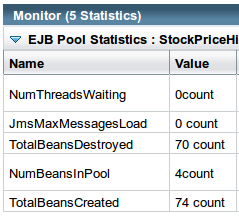
It is important to monitor statistics like this in order to understand the performance of applications, but be aware the monitoring itself imposes some cost. In this case, I set the GlassFish monitoring level for the EJB Container to HIGH to generate those statistics, and the total throughput dropped by about 5%. That’s a small price to pay for some visibility into an application, but for application servers that offer configurable monitoring, pay attention to what you need and configure monitoring accordingly. In the case of GlassFish, configuring the monitoring level to LOW has a negligible impact—that monitoring can be used for most operations, and monitoring can be dynamically set to HIGH when more information is required.
Or, frankly, I would recommend that it should be avoided in almost all cases. The usual argument for passivation is the scenario where the session is idle for hours or days at a time. When the user does come back (days later), you want her to find her state intact. The problem with that scenario is it assumes the EJB session is the only important state. Usually, though, the EJB is associated with an HTTP session, and keeping the session for days is not recommended. If the application server has a non-standard feature to store the HTTP session to disk, then a configuration where both the HTTP session and EJB session data is passivated at the same time (and for the same duration) may make sense. Even then, though, there is likely other external state as well.[60]
If long-lived state is required, you’ll usually need to bypass the normal Java EE state mechanisms.
Stateful beans that are assigned to a session are not held in the EJB pool; they are held in the EJB cache. Hence, the EJB cache must be tuned so that it is large enough to hold the maximum number of sessions expected to be active simultaneously in an application. Otherwise, the sessions which are least recently used will be passivated. Again, accomplishing this is different in different application servers. GlassFish sets a default value for the cache size of 512, and the value can be overridden globally in the domain configuration, or on a per-EJB basis in the sun-ejb-jar.xml file.
Quick Summary
- EJB caches are used only for stateful session beans while they are associated with an HTTP session.
- EJB caches should be tuned large enough to prevent passivation.
Local and Remote Instances
EJBs can be accessed via local or remote interfaces. In the canonical Java EE deployment, EJBs are accessed through servlets, and the servlet has the choice of using the local or remote interface to access the EJB. If the EJB is on another system, then of course the remote interface must be used, but if the EJB is co-located with the servlet (which is the more common deployment topology), the servlet should always use a local interface to access the EJB.
That may seem obvious, since a remote interface implies a network call. But that isn’t the reason—when the servlet and EJB are deployed in the same application server, most servers are smart enough to bypass the network call and just invoke the EJB method through normal method calls.
The reason to prefer local interfaces is the way in which the two interfaces handle their arguments. Arguments that are passed to (or returned from) a local EJB follow normal Java semantics: primitives are passed by value and objects are passed by reference.[61]
Arguments that are passed to (or returned from) a remote EJB must always be passed by value. That is the only possible semantic over a network: the sender serializes the object and transmits the byte stream, while the receiver deserializes the byte stream to reconstitute the object. Even when the server optimizes the local call by avoiding the network, it is not allowed to bypass the serialization/deserialization step.[62] No matter how well-written the server is, using a remote EJB interface within the server will always be slower than using a local one.
JavaEE offers other deployment scenarios. For example, the servlet and EJBs can be deployed in different tiers, and remote EJBs can be accessed from an ordinary application via their remote interface. There are often business or functional reasons that dictate the topology; for example, if the EJBs access corporate databases, you may want to run them on machines that are behind a separate firewall than the servlet container. Those reasons trump performance considerations. But from the strict perspective of performance, co-locating EJBs with whatever is accessing them and using local interfaces will always be faster than using a remote protocol.
Speaking of protocols: all remote EJBs must support the IIOP (CORBA) protocol. That is great for interoperability, particular with other programs that are not written in Java. Java EE server vendors are also allowed to use any other protocol, including proprietary ones, for remote access. Those proprietary protocols are invariably faster than CORBA (that is the reason the server vendors developed them in the first place). So when remote EJB calls must be used (and when interoperability is not a concern), explore the options for access protocols provided by the application server vendor.
Quick Summary
- Remote Interfaces impose a performance burden when calling EJBs, even within the same server.
XML and JSON Processing
When Java EE application servers host servlet-based applications to display their output in a browser, the data returned to the user is almost always HTML. This chapter has covered some best-practices of how to exchange that data.
Application servers are also used to exchange data with other programs, particularly via HTTP. Java EE supports different kinds of HTTP-based data transfer: full-blown webservice calls using the JAX-WS stack, RESTful calls using JAX-RS, and even simpler roll-your-own HTTP calls. The common feature of these APIs is that they utilize a text-based data transfer (based on either XML or JSON). Although they are quite different in their data representation, XML and JSON are similar in terms of how they are processed in Java, and the performance considerations of that processing is similar.
This is not meant to minimize the important functional differences between the two representations. As always, the choice of which representation to utilize should be based on algorithmic and programmatic factors rather than (solely) on their performance characteristics. If interoperability with another system is the goal, then the choice is dictated by that defined interface. In a complex program, dealing with traditional Java objects is often much easier than walking through document trees; in that case, JAXB (and hence XML) is the better option.[63]
There are other important functional differences between XML and JSON as well. So while this section makes some performance comparisons, the real goal here is to understand how to get the best possible performance out of whichever representation is chosen, rather than to drive a choice that might not be optimal for a particular environment.
Data Size
Basic Web Container Performance showed the effect of the size of data on overall performance. In a distributed network environment, that size is always important. In that regard, JSON is widely considered to be smaller than XML, though that difference is typically small. In the tests for this section, I used the XML and JSON returned from requesting the 20 most popular items from eBay. The XML in that example is 23,031 bytes, while the JSON is smaller at only 16,078 bytes. The JSON data has no whitespace at all, making it difficult for a human to read—which makes sense; human readability isn’t the goal. But oddly, the XML data is well-structured, with lots of white space; it could be trimmed to 20,556 bytes. Still that’s a 25% difference, which occurs mostly because of the XML closing tags. In general, those closing tags will always make the XML output larger.[64]
Whichever representation is used, both greatly benefit from enabling compression as they are transferred. In fact, once the data is compressed, the sizes are strikingly similar: 3,471 bytes for the compressed JSON data and 3,742 for the compressed XML file. That makes the size difference relatively unimportant, and the time to transmit the smaller compressed data will show the same benefit as transferring any other compressed HTTP data.
Quick Summary
- Like HTML data, programmatic data will greatly benefit from reducing whitespace and being compressed.
An Overview of Parsing and Marshalling
Given a series of XML or JSON strings, a program must convert those strings into data suitable for processing by Java. This is called either marshalling or parsing, depending on the context and the resulting output. The reverse—producing XML or JSON strings from other data—is called unmarshalling.
There are four general techniques to handle the data:
- Token Parsers
- A parser goes through the tokens of the input data and calls back methods on an object as it discovers tokens.
- Pull Parsers
- The input data is associated with a parser and the program asks for (or pulls) a series of tokens from the parser.
- Document Models
- The input data is converted to a document-style object which the application can then walk through as it looks for pieces of data.
- Object Representations
-
The input data is converted to one or more Java objects using a set of pre-defined classes that reflect the structure of the data (e.g., there will be a pre-defined
Personclass for data that represents an individual).
These techniques are listed in rough order of slowest to fastest, but again the functional differences between them are more important than their performance differences. There isn’t a great deal of functional difference between the first two; either parser is adaptable to most algorithms that need only to scan through the data once and pull out information. But simple scanning is all a parser can do. Parsers are not ideally suited for data that must be accessed in random order, or examined at more than once. To handle those situations, a program using only a simple parser would need to build some internal data structure—which is a simple matter of programming. But the document and Java object models already provide structured data, which may be easier than defining new structures on your own.
This, in fact, is the real difference between using a parser and using a data marshaller. The first two items in the list are pure parsers, and it is up to the application logic to handle the data as the parser provides it. The second two are data marshallers—they must use a parser to process the data, but they provide a data representation that more complex programs can use in their logic.
So the primary choice regarding which technique to use is determined by how
the application needs to be written. If a program needs to make one simple
pass through the data, then simply using the fastest parser will suffice.
Directly using a parser is also appropriate if the data is to be saved in
a simple, application-defined structure—e.g., the prices for the items
in the sample data could be saved to an
ArrayList, which would be
easy for other application logic to process.
Using a document model is more appropriate when the format of the data is important. If the format of the data must be preserved, then a document format is very easy: the data can be read into the document format, altered in some way, and then the document format can simply be written to a new data stream.
For ultimate flexibility, an object model provides Java-language level representation of the data. The data can be manipulated in the familiar terms of objects and their attributes. The added complexity in the marshalling is (mostly) transparent to the developer and may make that part of the application a little slower, but the productivity improvement in working with the code can offset that issue.
The goal in the examples used in this section is to take the 20-item XML or JSON document and save the item IDs into an array list. For some tests, only the first 10 items are needed. This emulates something often found in the real world—web interfaces often return more data than is actually needed. As a design consideration for a web service, that’s a good thing: the setup for the call takes some time, and it is better to have fewer remote calls (even if they retrieve too much data) than to make many fine-grained remote calls.
While all the examples show this common operation, the point is not to compare their performance directly on only that part of the task. Rather, each example will show how to perform the operation most efficiently within the chosen framework, since the choice of the framework will be driven by reasons other than the pure parsing and/or marshalling performance.
Quick Summary
- There are many ways for Java EE applications to process programmatic data.
- As these techniques provide more functionality to developers, the cost of the data processing itself will increase. Don’t let that dissuade you from choosing the right paradigm for handling the data in your application.
Choosing a parser
All programmatic data must be parsed. Whether applications use a parser directly, or indirectly by using a marshalling framework, the choice of the parser is important in the overall performance of the data operations.
Pull Parsers
From a developer’s perspective, it is usually easiest to use a pull parser. In the XML world, these are known as StAX (Streaming API for XML) parsers. JSON-P provides only a pull parser.
Pull parsers operate by retrieving data from the stream on demand. The basic pull parser for the tests in this section has this loop as its main logic:
XMLStreamReaderreader=staxFactory.createXMLStreamReader(ins);while(reader.hasNext()){reader.next();intstate=reader.getEventType();switch(state){caseXMLStreamConstants.START_ELEMENT:Strings=reader.getLocalName();if(ITEM_ID.equals(s)){isItemID=true;}break;caseXMLStreamConstants.CHARACTERS:if(isItemID){Stringid=reader.getText();isItemID=false;if(addItemId(id)){return;}}break;default:break;}}
The parser returns a series of tokens. In the example most tokens are
just discarded. When a start token is found, to code checks to see if the
token is an item ID.
If it is, then the next character token will be the ID the application
wants to save.
The ID is saved via the
addItemId() method, which
returns true
if the desired number
of IDs have been stored. When that happens, the loop can just return and not
process the remaining data in the input stream.
Conceptually, the JSON parser works exactly the same way; only some of the API calls have changed:
while(parser.hasNext()){Eventevent=parser.next();switch(event){caseKEY_NAME:Strings=parser.getString();if(ITEM_ID.equals(s)){isItemID=true;}break;caseVALUE_STRING:if(isItemID){if(addItemId(parser.getString())){return;}isItemID=false;}continue;default:continue;}}
Processing only the necessary data here gives a predictable performance benefit. Table 10-3 shows the average time in milliseconds to parse the sample document assuming parsing stops after ten items, and to process the entire document. Stopping after finding ten items does not save 50% of the time (because there are other sections of the document that still get parsed), but the difference is still significant.
Push Parsers (SAX)
The standard XML parser is a SAX (Simple API for XML) parser. The SAX parser is a push parser: it reads the data and when it finds a token, executes a callback to some class that is expected to handle the token. The parsing logic for the test remains the same, but the logic now appears in callback methods defined in a class:
protectedclassCustomizedInnerHandlerextendsDefaultHandler{publicvoidstartElement(Stringspace,Stringname,Stringraw,Attributesatts){if(name.length()==0)name=raw;if(name.equalsIgnoreCase(ITEM_ID))isItemID=true;}publicvoidcharacters(char[]ch,intstart,intlength)throwsSAXDoneException{if(isItemID){Strings=newString(ch,start,length);isItemID=false;if(addItemId(s)){thrownewSAXDoneException("Done");}}}}
The only difference in the program logic here is an exception must be thrown
to signal that parsing
is completed, since that’s the
only way the XML push parsing framework can detect that parsing should stop.
The application-defined
SAXDoneException
is the class this example defines for that case. In general any
kind of
SAXException
can be thrown—this example uses a subclass so that the
rest of the program logic can differentiate between an actual error and
the signal that processing should stop.
SAX parsers tend to be faster than StAX parsers, though the performance difference is slight—the choice is which parser to use should be made based on which model is easiest to use in development. Table 10-4 shows the difference in processing time between the push and pull parsers.
| Items Processed | XML StAX Parser | XML SAX Parser |
10 | 143 ms | 132 ms |
20 | 265 ms | 231 ms |
There is no corresponding push parser model for JSON-P.
Alternate Parsing Implementations and Parser Factories
The XML and JSON specifications define a standard interface for parsers. The JDK provides a reference implementation of the XML parser, and the JSON-P project (http://jsonp.java.net) provides a reference implementation of the JSON parser. Applications can use any arbitrary parser (as long as the parser implements the desired interfaces, of course).
Parsers are obtained via a parser factory. Using a different parser implementation is a matter of configuring the parser factory to return an instance of the desired parser (rather than the default parser). There are a few performance implications around this:
- Factory instantiation is expensive: make sure the factory is reused via a global (or at least a thread local) reference.
- The configuration of the factory can be achieved in different ways, some of which (including the default mechanism) can be quite suboptimal from a performance standpoint.
- Different parser implementations may be faster than the default ones.
Let’s look at those points in order.
In these tests, the data stream is parsed 1,000,000 times in order to find the average parsing speed (after a warmup period of 10,000 parses). The example code needs to make sure it constructs the factory only once, which is done in an initialization method called at the beginning of the test. The actual parser for each test is then retrieved via the factory on demand. Hence the SAX test contains this code:
SAXParserFactoryspf;// Called once on program initializationprotectedvoidengineInit(RunParamsrp)throwsIOException{spf=SAXParserFactory.newInstance();}// Called each iterationprotectedXMLReadergetReader()ThrowsSAXException{returnspf.newSAXParser().getXMLReader();}
The StAX parser looks similar, though the factory (of type
XMLInputFactory)
is returned from calling
the
XMLFactory.newInstance()
method, and the reader is
returned from calling the
createStreamReader()
method. For JSON,
the corresponding calls are the
Json.createParserFactory()
and
createParser()
methods.
To use a different parser implementation, we must start with a different factory, so that the call to the factory returns the desired implementation. This brings us to the second point about factory configuration: make sure the factory to use is optimally specified.
XML factories are specified by setting a property in one of three ways.
The property used in the discussion here
(javax.xml.stream.XMLInputFactory)
is the property for
the default StAX parser. To override the default SAX parser,
the property in question is
javax.
xml.
parsers.
SAXParserFactory
.
In order to determine which factory is in use, the following options are searched in order:
-
Use the factory specified by the system property
-Djavax.xml.stream.XMLInputFactory=my.factory.class. Use the factory specified in the file called called jaxp.properties in the JAVA/jre/lib directory. The factory is specified by a line like this:
javax.xml.stream.XMLInputFactory=my.factory.class
-
Search the classpath for a file called
META-INF/services/javax.xml.stream.XMLInputFactory. The file should contain
the single line
my.factory.pass:[class. - Use a JDK-defined default factory.
The third option can have a significant performance penalty, particularly in an environment where there is a very lengthy classpath. To see if an alternate implementation has been specified, each entry in the classpath must be scanned for the appropriate file in the META-INF/services directory. That search is repeated every time a parser is created, so if the classloader does not cache the lookup of that resource (and most classloaders do not), instantiating parsers will be very expensive.
It is much better to use one of the first two options to configure your application. The options in the list work in order; once the parser is found, searching stops.
The downside of those first two options is that they apply globally to all code in the application server. If two different EE applications are deployed to the same server and each requires a different parser factory, the server must rely on the (potentially slow) classpath technique.
The way that the parser factory is found affects even the default factory: the JDK can’t know to use the default factory until it searches the classpath. Hence, even if you want to use the default factory, you should configure the global system property or JRE property file to point to the default implementation. Otherwise, the default parser (choice four in the list) won’t be used until the expensive search in step three has been made.
For JSON, the configuration is a slightly different: the only way to specify an alternate implementation is to create one using the META-INF/services route, specifying a file with the name javax.json.spi.JsonProvider that contains the classname of the new JSON implementation. There is (unfortunately) no way to circumvent searching the entire classpath when looking for a JSON parser.
The final performance consideration in choosing a parser is the performance of the alternate implementation. This section can only give a snapshot of the performance of some implementations here; don’t necessarily take the results at face value. The point is that there will always be different parser implementations. In terms of performance, different implementations will likely leapfrog the performance of each other. At some point in time, alternate parsers will be faster than the reference implementations (possibly until new releases of the JDK or JSON-P reference implementation come along and leapfrog the alternate implementation).
At the time of this writing, for example, the alternate Woodstox parser (http://woodstox.codehaus.org/) provides a slightly faster implementation of the StAX parser than what ships with JDK 7 and 8:
| Items Processed | JDK StAX Parser | Woodstox StAX Parser |
10 | 143 ms | 125 ms |
20 | 265 ms | 237 ms |
The JSON situation is more muddled. As I write this, the JSON-P specification has just been made final, and there are no JSR 353-compatible alternate implementations of JSON parsers. There are other parsers for JSON, and it is only a matter of time until at least some of them conform to the JSR 353 API.
This is a fluid situation, so it may be a good idea to look for alternate JSON implementations and see if they offer better performance. One (currently non-compliant) implementation is the Jackson JSON processor (https://github.com/FasterXML/jackson) which already implements a basic pull parser (just not the exact API calls of JSR 353).
| Items Processed | JavaEE JSON Parser | Jackson JSON Parser |
10 | 68 ms | 40 ms |
20 | 146 ms | 74 ms |
This is a usual situation for new JSR reference implementations; just as the JDK 7 XML parser is much faster than previous versions, new JSON-P parsers will can be expected to show large performance gains as well.[65]
Quick Summary
- Choosing the right parser can have a big impact on performance of an application.
- Push parsers tend to be faster than pull parsers.
- The algorithm used to find the factory for a parser can be quite time-consuming; if possible, bypass the services implementation and specify a factory directly via a system property.
- At any point in time, the winner of the fastest parser implementation race may be different. Seek out alternate parsers when appropriate.
XML Validation
XML data can optionally be validated against a schema. This allows the parser to reject a document that isn’t well-formed—meaning one that is missing some required information, or one that contains some unexpected information. “Well-formed” is used here in terms of the content of the document; if the document has a syntax error (e.g., content not within an XML tag, or a missing XML closing tag, etc.), then all parsers will reject the document.
This validation is one benefit XML has over JSON. You can supply your own validation logic when parsing JSON documents, but with XML, the parser can perform the validation for you. That benefit is not without its cost in terms of performance.
XML validation is done against one more more schema or DTD files. Although validating against DTDs is faster, XML schemas are more flexible, and their use now predominates in the XML world. One thing that makes schemas slower than DTDs is that schemas are usually specified in different files. So the first thing that can be done to reduce the penalty for validation is to consolidate the schema files: the more schema files that need to be processed, the more expensive validation is. There is a trade-off here between the maintainability of the separate files and the performance gain involved. Unfortunately, schema files are not easy to combine (e.g., like CSS or javascript files are), since they maintain different namespaces.
The location from which schema files are loaded can be a significant source of performance issues. If a schema or DTD must be repeatedly loaded from the network, performance will suffer. Ideally, the schema files should be delivered along with the application code so that the schema(s) can be loaded from the local filesystem.
For normal validation with SAX,[66] the code simply sets some properties on the SAX parser factory:
SAXParserFactoryspf=SAXParserFactory.newInstance();spf.setValidating(true);spf.setNamepsaceAware(true);SAXParserparser=spf.newSAXParser();// Note: above lines can be executed once to create a parser. If// reusing a parser, instead call parser.reset() and then set its// propertiesparser.setProperty(JAXPConstants.JAXP_SCHEMA_LANGUAGE,XMLConstants.W3C_XML_SCHEMA_NS_URI);XMLReaderxr=parser.getXMLReader();xr.setErrorHandler(newMyCustomErrorHandler());
The default for the parser is for it to be non-validating, so the first call
that is needed is to the
setValidating
method. Then a property must be
set to tell the parser
which language to validate against—in this case, the W3C XML schema
language (e.g., XSD files). Finally, all validating parsers must set an error
handler.
This processing—the default way to process the XML document—will re-read the schema each time a new document is parsed, even if the parser itself is being reused. For additional performance, consider reusing schemas.
Reusing schemas provides an important benefit even when the schema is loaded from the filesystem. When loaded, the schema must itself be parsed and processed (it is an XML document, after all). Saving the results of this processing it and reusing it will give a big boost to XML processing. This is particularly true in the most common use case: that the application receives and processes thousands of XML documents, all of which conform to the same (set of) schema(s).
There are two options for reusing a schema. The first option (which works only for the SAX parser) is to create schema objects and associate them with the parser factory:
SchemaFactorysf=SchemaFactory.newInstance(XMLConstants.W3C_XML_SCHEMA_NS_URI);StreamSourcess=newStreamSource(rp.getSchemaFileName());Schemaschema=sf.newSchema(newSource[]{ss});SAXParserFactoryspf=SAXParserFactory.newInstance();spf.setValidating(false);spf.setNamespaceAware(true);spf.setSchema(schema);parser=spf.newSAXParser();
Note that the
setValidating()
method is called with a parameter of false
in this case. The
setSchema()
and
setValidating()
methods are mutually
exclusive ways of performing schema validation.
The second option for reusing schema objects is to use an instance of the
Validator
class. That allows parsing to be separated from
validation, so the two operations can be performed at different times.
When used with the StAX
parser, this also allows validation to be performed during parsing by
embedding a special reader into the validation stream.
To use a
Validator,
first create that special reader. The logic of the
reader is the same
as before: it looks for the
itemID
start element and saves those
IDs when they are found. However, it must do this by acting as a delegate
to a default StAX stream reader:
privateclassMyXMLStreamReaderextendsStreamReaderDelegate(){XMLStreamReaderreader;publicMyXMLStreamReader(XMLStreamReaderxsr){reader=xsr;}publicintnext()throwsXMLStreamException{intstate=super.next();switch(state){caseXMLStreamConstants.START_ELEMENT:...processthestartelementlookingforItemID...break;caseXMLStreamConstants.CHARACTERS:...ifitemid,savethecharacters.break;}returnstate;}}
Next, associate this reader with the input stream that the
Validator
object will use:
SchemaFactorysf=SchemaFactory.newInstance(XMLConstants.W3C_XML_SCHEMA_NS_URI);StreamSourcess=newStreamSource(rp.getSchemaFileName());Schemaschema=sf.newSchema(newSource[]{ss});XMLInputFactorystaxFactory=XMLInputFactory.newInstance();staxFactory.setProperty(XMLInputFactory.IS_VALIDATING,Boolean.FALSE);XMLStreamReaderxsr=staxFactory.createXMLStreamReader(ins);XMLStreamReaderreader=newMyXMLStreamReader(xsr);Validatorvalidator=schema.newValidator();validator.validate(newStAXSource(newStaxSource(reader)));
The
validate()
method, while performing regular validation, will also
call the stream reader delegate, which will parse the
desired information from the input data (essentially, as a side-effect
of validation).
One downside to this approach is that
processing cannot be cleanly terminated once the ten items have been read.
The code can still throw an exception
from the
next()
method and catch that exception later—just as was
previously done for the
SAXDoneException.
The problem is that
the default schema listener will print out an error message during processing
when the exception is thrown.
Table 10-7 shows the effect of all these operations. Compared to simple (non-validating) parsing, parsing with the default validation incurs a large penalty. Reusing the schema makes up some of that penalty and gives us the assurance that the XML document in question is well-formed, but validation always carries a significant price.
| Parsing Mode | SAX | StAX |
No Validation | 231 ms | 265 ms |
Default Validation | 730 ms | N/A |
Schema Reuse | 649 ms | 1392 ms |
Quick Summary
- When schema validation is functionally important, make sure to use it; just be aware that it will have a significant performance penalty to parsing the data.
- Always reuse schemas to minimize the effect of validation.
Document Models
Building a DOM or JSON object is a relatively simply series of calls. The object itself is created with an underlying parser, so it is important to configure the parser for optimal performance (in the case of DOM, the StAX parser is used by default).
DOM objects are created with a
DocumentBuilder
object which is
retrieved from the
DocumentBuilderFactory.
The default document builder
factory is specified via the
javax.xml.parsers.DocumentBuilderFactory
property (or the META-INF/services file of that name). Just as it is
important to configure a property for optimal performance when
creating a parser, it is important to configure that system property
for optimal
performance when creating document builders.
Like SAX parsers,
DocumentBuilder
objects can be reused as long as their
reset()
method is called in between uses.
JSON objects are created with a
JsonReader
object which is retrieved
from the
Json
object directly
(by calling the
Json.createReader()
method) or from a
JsonReaderFactory
object (by calling the
Json.createJsonReaderFactory()
method).
The reader factory can be configured via a
Map
of properties, although
the JSR 353 RI does not presently support any configuration
options.
JsonReader
objects are not reusable.
Document/object models are expensive to create compared to simply parsing the corresponding data:
| Time Required to | XML | JSON |
Parse Data | 265 ms | 146 ms |
Build Document | 348 ms | 197 ms |
The time to build the document includes parsing time, plus the time to create the document/object structure—so it can be inferred from this table that the time to create the structure is roughly 33% of the total time for XML, and 25% of the total time of JSON. More complicated documents may show a larger percentage of time spent building the document model.
The previous parsing tests were sometimes only interested in the first ten items. If the object representation similarly should contain only the first ten items, then there are two choices. First, the object can be created, and then various methods can be used to walk through the object and discard any undesired items. That is the only option for JSON objects.
DOM objects can set up a filtering parser using DOM level 3 attributes. This first requires that a parsing filter be created:
privateclassInputFilterimplementsLSParserFilter{privatebooleandone=false;privatebooleanitemCountReached;publicshortacceptNode(Nodenode){if(itemCountReached){Strings=node.getNodeName();if("ItemArray".equals(s)){returnNodeFilter.FILTER_ACCEPT;}if(done){returnNodeFilter.FILTER_SKIP;}// This is the </Item> element// the last thing we needif("Item".equals(s)){done=true;}}returnNodeFilter.FILTER_ACCEPT;}publicintgetWhatToShow(){returnNodeFilter.SHOW_ALL;}publicshortstartElement(Elementelement){if(itemCountReached){returnNodeFilter.FILTER_ACCEPT;}Strings=element.getTagName();if(ITEM_ID.equals(element.getTagName())){if(addItemId(element.getNodeValue())){itemCountReached=true;}}returnNodeFilter.FILTER_ACCEPT;}}
The parsing filter is called twice for each element: the
startElement()+
method is called when parsing of an element begins, and the
acceptNode()
method is called when parsing of an element is finished. If
the element in question should not be represented in the final DOM document,
one of those methods should return
FILTER_SKIP.
In this case, the
startElement()
method is used to keep track of how many items have been
processed, and the
acceptNode()
method is used to determine whether the
entire element should
be skipped or not. Note that the code must also keep track of the
ending
<Item>
tag so as not to skip that. Also notice that only elements of
type
ItemArray
are skipped; the XML document has other elements in it
that should not be skipped.
To setup the input filter, the following code is used:
System.setProperty(DOMImplementationRegistry.PROPERTY,"com.sun.org.apache.xerces.internal.dom.DOMImplementationSourceImpl");DOMImplementationRegistryregistry=DOMImplementationRegistry.newInstance();DOMImplementationdomImpl=registry.getDOMImplementation("LS 3.0");domLS=(DOMImplementationLS)domImpl;LSParserlsp=domLS.createLSParser(DOMImplementationLS.MODE_SYNCHRONOUS,"http://www.w3.org/2001/XMLSchema");lsp.setFilter(newInputFilter());LSInputlsi=domLS.createLSInput();lsi.setByteStream(is);Documentdoc=lsp.parse(lsi);
In the end, a
Document
object is created, just as it would have been
without filtering the input—but in this case, the resulting document
is much smaller. That
is the point of filtering: the actual parsing and filtering will take much
longer to produce the a filtered document than a document that contains
all the original data. Because the document occupies less
memory, it is a useful technique if the document will be long-lived (or if
there are many such documents in use), since it reduces pressure on the
garbage collector.
Table 10-9 shows the difference for parsing speeds of the usual XML file when constructing a DOM object representing only half (10) of the items.
| Standard DOM | Filtering DOM | |
Time to create DOM | 348 ms | 417 ms |
Size of DOM | 101,440 bytes | 58,824 bytes |
Quick Summary
-
DOM and
JsonObjectmodels of data are more powerful to work with than simple parsers, but the time to construct the model can be significant. - Filtering data out of the model will take even more time than constructing the default model, but that can still be worthwhile for long-lived or very large documents.
Java Object Models
The final option in handling textual data is to create a set of Java classes that correspond to the data being parsed. There are JSR proposals for doing this in JSON, but no standard. For XML, this is accomplished using JAXB.
JAXB uses an underlying StAX parser, so configuring the best StAX
parser for your platform will help JAXB performance. The Java objects
created via JAXB come from creating an
Unmarshaller
object:
JAXBContextjc=JAXBContext.newInstance("net.sdo.jaxb");Unmarshalleru=jc.createUnmarshaller();
The
JAXBContext
is expensive to create. Fortunately,
it is thread safe: a single global context can be created
and reused (and sharing among threads).
Unmarshaller
objects are
not thread safe; a new one must be created for each thread. However,
the unmarshaller can be reused, so keeping one in a thread local (or keeping
a pool of them) will help performance when processing lots
of documents.
Creating objects via JAXB is more expensive than either parsing or creating a DOM document. The trade-off is that using those objects is much faster than walking through a document (not to mention that using the objects is a simple matter of writing regular Java code, instead of the convoluted API used to access documents). In addition, writing out the XML that a set of JAXB documents represents is much faster than writing out the XML from a document. Table 10-10 shows the performance differences for the sample 20-item document.
| Marshall | Unmarshall | |
DOM | 348 ms | 298 ms |
JAXB | 414 ms | 232 ms |
Quick Summary
- For XML documents, producing Java objects via JAXB yields the simplest programming model for accessing and using the data.
- Creating the JAXB objects will be more expensive than creating a DOM object model.
- Writing out XML data from JAXB objects will be faster than writing out a DOM object.
Object Serialization
XML, JSON, and similar text-based formats are useful for exchanging data between different kinds of systems. Between Java processes, data is typically exchanged by sending the serialized state of an object. Although it is used extensively throughout Java, serialization plays two important considerations in Java EE:
- EJB calls between Java EE servers—remote EJB calls—use serialization to exchange data
- HTTP session state is saved via object serialization, which enables HTTP sessions to be highly-available.
The JDK provides a default mechanism to serialize objects that
implement either the
Serializable
or
Externalizable
interface.
The serialization performance of practically every object
imaginable can be improved from the default serialization code, but this is
definitely one of those times when it would be unwise
to perform that optimization prematurely. The special code to serialize and
deserialize the object will take a fair amount of time to write,
and the code will be
harder to maintain than code that uses default serialization.
Serialization code
can also be a little tricky to write correctly, so attempting to optimize it
increases the risk of producing incorrect code.
Transient Fields
In general, the way to improve object serialization cost is to serialize
less data. This is done by marking fields as
transient,
in which case
they are not serialized by default.
Then the class can supply special
writeObject()
and
readObject()
methods
to handle that data.[67]
Overriding Default Serialization
The
writeObject()
and
readObject()
methods allow complete control over how data is serialized. With great
control comes great responsibility: it’s easy to get this wrong.
To get an idea of why serialization optimizations are tricky, take
the case of a simple Point object that represents a location:
publicclassPointimplementsSerializable{privateintx;privateinty;...}
On my machine, 100,000 of these objects can be serialized in 133 milliseconds, and deserialized in 741 milliseconds. But even as simple as that object is, it could—if very, very hard pressed for performance—be improved:
publicclassPointimplementsSerializable{privatetransientintx;privatetransientinty;....privatevoidwriteObject(ObjectOutputStreamoos)throwsIOException{oos.defaultWriteObject();oos.writeInt(x);oos.writeInt(y);}privatevoidreadObject(ObjectInputStreamois)throwsIOException,ClassNotFoundException{ois.defaultReadObject();x=ois.readInt();y=ois.readInt();}}
Serializing 100,000 of these objects on my machine still takes 132 milliseconds, but deserializing them takes only 468 milliseconds—a 30% improvement. If serializing a simple object is what takes a significant portion of time in a program, then it might make sense to optimize it like this. Be aware, however, that it makes the code harder to maintain as fields are added, moved, and so on.
So far, though, the code is more complex but is still functionally correct (and faster). But beware of using this technique in the general case:
publicclassTripHistory{privatetransientPoint[]airportsVisited;....// THIS CODE IS NOT FUNCTIONALLY CORRECTprivatevoidwriteObject(ObjectOutputStreamoos)throwsIOException{oos.defaultWriteObject();oos.writeInt(airportsVisited.length);for(inti=0;i<airportsVisited.length;i++){oos.writeInt(airportsVisited[i].getX());oos.writeInt(airportsVisited[i].getY());}}privatevoidreadObject(ObjectInputStreamois)throwsIOException,ClassNotFoundException{ois.defaultReadObject();intlength=ois.readInt();airportsVisited=newPoint[length];for(inti=0;i<length;i++){airportsVisited[i]=newPoint(ois.readInt(),ois.readInt();}}}
Here, the
airportsVisited
field is an array of all the airports I’ve
ever flow to or from, in the order in which I visited them. So certain
airports, like JFK, appear frequently in the array; SYD appears only once
(so far).
Because it is expensive to write object references, this code would
certainly perform faster than the default serialization mechanism for that
array: an array of 100,000
Point
objects takes 4.7 seconds to serialize
on my machine and 6.9 seconds to deserialize. Using the above “optimization,”
it takes only 2 seconds to serialize and 1.7 seconds to deserialize.
This code, however, is incorrect. The references in the array that specify the location of JFK all started out referring to the same object. That means when I discover that the location represented in that data is incorrect, the single JFK reference can be changed, and all objects in the array will reflect that change (since they are references to the same object).
When the array is deserialized by the above code, those JFK references end up as separate, different objects. Now when one of those objects is changed, only that object is changed, and it ends up with different data than the remaining objects that refer to JFK.
This is a very important principle to keep in mind, because optimizing serialization is often about performing special handling for object references. Done correctly, that can greatly increase the performance of serialization code. Done incorrectly, it can introduce quite subtle bugs.
With that in mind, let’s explore the serialization of the
StockPriceHistory
class to see how serialization optimizations can be made. The fields in
that class include the following:
publicclassStockPriceHistoryImplimplementsStockPriceHistory{privateStringsymbol;protectedSortedMap<Date,StockPrice>prices=newTreeMap<>();protectedDatefirstDate;protectedDatelastDate;protectedbooleanneedsCalc=true;protectedBigDecimalhighPrice;protectedBigDecimallowPrice;protectedBigDecimalaveragePrice;protectedBigDecimalstdDev;privateMap<BigDecimal,ArrayList<Date>>histogram;....publicStockPriceHistoryImpl(Strings,DatefirstDate,DatelastDate){prices=....}}
When the history for a stock is constructed for a given symbol s, the
object creates and stores a sorted map of
prices
keyed by date of all
the prices between
start and
end.
The code also saves the
firstDate
and the
lastDate.
The
constructor doesn’t fill in any other fields; they are initialized lazily.
When a getter on any of those fields is called, the getter
checks if
needsCalc
is
true.
If it is, it calculates the appropriate
values for the remaining fields if necessary (all at once).
This calculation includes creating the
histogram,
which
records how many days the stock closed at a particular price. The histogram
contains the same data (in terms of
BigDecimal
and
Date
objects)
as is found in the
prices
map; it is just a different way of looking
at the data.
Because all of the lazily-initialized fields can be calculated from
the
prices
array, they can all be marked
transient,
and no special work
is required to serialize or deserialize them. The example is easy in this
case because the code was already doing lazy initialization of the fields;
it can repeat that lazy initialization when receiving the data.
Even if the code eagerly initialized these fields, it could still
mark
any calculated fields
transient
and recalculate their values in the
readObject()
method of the class.
Note too that this preserves the object relationship between the
prices
and
histogram
objects: when the histogram is recalculated, it will
just insert existing objects into the new map.
This kind of optimization is almost always a good thing, but there are
cases when it can actually hurt performance. Table 10-11
shows the time it takes to serialize and deserialize this case where the
histogram
object is transient vs. non-transient, as well as the size
of the serialized data for each case.
| Object | Serialization Time | Deserialization Time | Size of Data |
No transient fields | 12.8 seconds | 11.9 seconds | 46,969 bytes |
Transient histogram | 11.5 seconds | 10.1 second | 40,910 bytes |
So far, the example saves about 15% of the total time to serialize and
deserialize the object. But this test has not actually recreated
the
histogram
object on the receiving side: that object will be created
when the receiving code first accesses it.
There are times that the
histogram
object
will not be needed: the client may only be interested in the prices
on particular days, and not the histogram. That is where the more
unusual case comes in: if the
histogram
will always be needed, and if it takes
more than 3.1 seconds to calculate all the histograms in this test, then
the case with the lazily-initialized fields will actually have
a net performance decrease.
In this case, calculating the histogram does not fall into that category—it is a very fast operation. In general, it may be hard to find a case where recalculating a piece of data is more expensive than serializing and deserializing that data. But it is something to consider as code is optimized.
This test is not actually transmitting data; the data is
written to and read from pre-allocated byte arrays, so that it measures
only the time for serialization and deserialization. Still,
notice that making the
histogram
field transient has also
saved about 13% in the size of the data. That will be quite important if
the data is to be transmitted via a network.
Compressing Serialized Data
This leads to a third way in which serialization performance of code can be improved: compress the serialized data so that it is faster to transmit over a slow network. In the stock history class, that is done by compressing the prices map during serialization:
publicclassStockPriceHistoryCompressimplementsStockPriceHistory,Serializable{privatebyte[]zippedPrices;privatetransientSortedMap<Date,StockPrice>prices;privatevoidwriteObject(ObjectOutputStreamout)throwsIOException{if(zippedPrices==null){makeZippedPrices();}out.defaultWriteObject();}privatevoidreadObject(ObjectInputStreamin)throwsIOException,ClassNotFoundException{in.defaultReadObject();unzipPrices();}protectedvoidmakeZippedPrices()throwsIOException{ByteArrayOutputStreambaos=newByteArrayOutputStream();GZIPOutputStreamzip=newGZIPOutputStream(baos);ObjectOutputStreamoos=newObjectOutputStream(newBufferedOutputStream(zip));oos.writeObject(prices);oos.close();zip.close();zippedPrices=baos.toByteArray();}protectedvoidunzipPrices()throwsIOException,ClassNotFoundException{ByteArrayInputStreambais=newByteArrayInputStream(zippedPrices);GZIPInputStreamzip=newGZIPInputStream(bais);ObjectInputStreamois=newObjectInputStream(newBufferedInputStream(zip));prices=(SortedMap<Date,StockPrice>)ois.readObject();ois.close();zip.close();}}
The
zipPrices()
method serializes the map of prices to a byte array
and saves the resulting bytes, which are then serialized normally in the
writeObject()
method when it calls the
defaultWriteObject()
method.[68] On deserialization, the reverse operation
is performed.
If the goal is to serialize to a byte stream (as in the original sample code), this is a losing proposition. That isn’t surprising; the time required to compress the bytes is much longer than the time to write them to a local byte array. Those times are shown in Table 10-12.
| Use Case | Serialization Time | Deserialization Time | Size of Data |
No Compression | 12.1 seconds | 8.0 seconds | 41,170 bytes |
Compression/Decompression | 26.8 seconds | 12.7 seconds | 5,849 bytes |
Compression Only | 26.8 seconds | 0.494 seconds | 5,849 bytes |
The most interesting point about this table is the last line. In that
test, the data
is compressed before sending, but the
unzipPrices()
method isn’t called
in the
readObject()
method. Instead, it is called when needed, which will be
the first time the client calls the
getPrice()
method. Absent that call, there are only a few
BigDecimal
objects to deserialize, which is quite fast.
It is quite possible in this
example that the client will never need the actual prices: the client may
only need to
call the
getHighPrice()
and similar methods to retrieve aggregate information
about the data. As long as those methods are all that is needed,
a lot of time can be saved by lazily decompressing the
prices
information.
This lazy decompression is also quite useful if the object in question is
being persisted—e.g., if it is HTTP session state that is being stored
as a backup copy in case the application server fails. Lazily decompressing
the data saves both CPU time (from skipping the decompression) and memory
(since the compressed data takes up less space).
So even if the application runs on a local, high-speed network—and particularly if the goal is to save memory rather than time—compressing data for serialization and then lazily decompressing it can be quite useful.
If the point of the serialization is to transfer data over the network, then the compression will win anytime there is data savings. Table 10-13 performs the same serialization for the 10,000 stock objects, but this time it transmits the data to another process. The other process is either on the same machine, or on a machine accessed via my broadband connection.
| Object | Same Machine | Broadband WAN |
No Compression | 30.1 seconds | 150.1 seconds |
Compression/Decompression | 41.3 seconds | 54.3 seconds |
Compression Only | 28.0 seconds | 44.1 seconds |
The fastest possible network communication is between two processes on the same machine—that communication doesn’t go onto the network at all, though it does send data through the operating system interfaces. Even in that case, compressing the data and lazily decompressing it has resulted in the fastest performance (at least for this test—smaller data amount may still show a regression). And the order of magnitude difference in the amount of data has made a (predictably) large difference in the total time once a slower network is involved.
Keeping Track of Duplicate Objects
This section began with an example of how not to serialize data that
contains object references, lest the object references be compromised when
the data is deserialized. However, one of the more powerful optimizations
possible in the
writeObject()
method is to not write out duplicate object
references. In the case of the
StockHistory
class, that means not writing
out the duplicate references of the
prices
map. Because the example uses a
standard JDK class for that map, we don’t have to worry about that:
the JDK classes
are already written to optimally serialize their data. Still, it is
instructive to look into how those classes perform their optimizations
in order to understand what is possible.
In the
StockHistoryImpl
class, the key structure is a
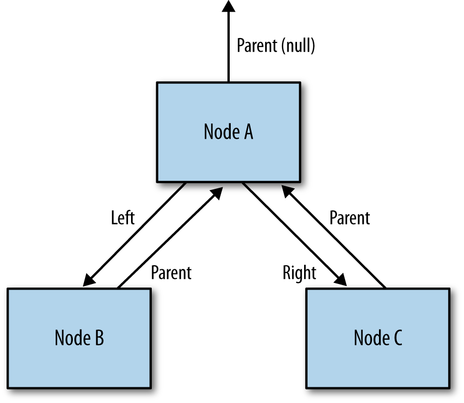
TreeMap.
A simplified version of that map appears in Figure 10-2. With default
serialization, the JVM would write out the primitive data fields for Node A;
then it would recursively call the
writeObject()
method for node B (and then
for node C). The code for Node B would write out its primitive data fields,
and then recursively write out the data for its
parent
field.
But wait a
minute—that
parent
field is Node A, which has already been written. The object
serialization code is smart enough to realize that: it doesn’t re-write the
data for Node A. Instead, it simply adds an object reference
to the previously-written data.
Keeping track of that set of previously-written objects, as well as all that
recursion, adds a small performance hit to object serialization. However,
as demonstrated in the example with an array of
Point
objects, it can’t
be avoided: code must keep
track of the previously-written objects and reconstitute the correct
object references. However, it is possible to perform smart
optimizations by suppressing object references that
can be easily re-created when the object is deserialized.
Different collection classes handle this differently. The
TreeMap
class,
for example, simply iterates through the tree and writes only the keys
and values; serialization discards all information about the relationship
between the keys (i.e., their sort order). When then data has been
deserialized, the
readObject()
method then re-sorts the data to produce a tree. Although sorting the
objects again sounds like
it would be expensive, it is not: that process is about 20% faster on a
set of 10,000 stock objects than
using the default object serialization which chases all the object
references.
The
TreeMap
class also benefits from this optimization because it can
write out fewer objects. A node (or in JDK language, an
Entry)
within a map
contains two objects: the
key and the value. Because the map cannot contain two identical nodes,
the serialization code doesn’t need to worry about preserving object
references to nodes. In this case, it can skip writing the node object itself,
and simply write the key and and value objects directly. So the
writeObject()
method ends up looking something like this (syntax adapted
for ease of reading):
privatevoidwriteObject(ObjectOutputStreamoos)throwsIOException{....for(Map.Entry<K,V>e:entrySet()){oos.writeObject(e.getKey());oos.writeObject(e.getValue());}....}
This looks very much like the code that didn’t work for the
Point
example.
The difference
in this case is that the code is still writing objects where those objects
can be the same.
A
TreeMap
cannot have two nodes that are the same, so there is no need to write out
node references. The
TreeMap
can have two values that are the same, so the values must be written out
as object references.
This brings us full-circle: as I stated at the beginning of this section, getting object serialization optimizations correct can be tricky. But when object serialization is a significant bottleneck in an application, optimizing it correctly can offer important benefits.
Quick Summary
- Serialization of data, particularly within Java EE, can be a big performance bottleneck.
-
Marking instance variables
transientwill make serialization faster and reduce the amount of data to be transmitted. Both of those are usually big performance wins, unless recreating the data on the receiver takes a very long time. -
Other optimizations via the
writeObject()andreadObject()methods can significantly speed up serialization. Approach them with caution, since it is easy to make a mistake and introduce a subtle bug. - Compressing serialized data is often beneficial, even if the data will not travel across a slow network.
Java EE Networking APIs
The data exchange techniques that we have just examined—XML parsing, JSON processing, and object serialization—have their uses within a variety of applications, but one of their primary uses is within one of the Java EE networking APIs: JAX-WS, JAX-RS, and IIOP/RMI.
These are very different protocols with very different features. Their feature set is the primary determinant of why and when you would use each of them. There are endless debates, for example, about whether JAX-RS is faster than JAX-WS, but those debates of necessity assume a common denominator application that can be written in either framework. If certain security features are required, then the choice will be JAX-WS, regardless of its relative performance to JAX-RS. If an application must talk to an existing server that exports an IIOP interface, then that dictates the choice.
As a set, though, the networking APIs have similar performance challenges to overcome. This section discusses some of those similar challenges and addresses how to meet them.
Sizing Data Transfers
The primary factor driving performance of these technologies is their data exchange, which is one reason this chapter spent a lot of time looking into that. The amount of data transfer should be minimized, whether by compression, or pruning of documents, or some other technique.
On the other hand, setting up a network call in the first place has a measurable overhead. When designing a network interface, the interface should be “coarse”—that is, it is better to return lots of data in one call, so as to minimize the total number of network calls that the client must make. That principle is at odds with the idea to reduce the amount of data being exchanged; some balance must be struck here.
This balance can be observed if we test the average response time for a RESTful webservice based on the stock history class. The service can be designed to return either just the basic data (high, low, average, and standard deviation) for the period, or to return the basic data plus all the individual daily data points.
If it is known ahead of time how the client will use the data, then it is easy to know exactly which data to return. However, that isn’t always possible. In this example, say that the client requests a five-year history for a stock, and the client application will initially just present a summary of that data to the user. What happens if the user wants to drill into that data and look at individual daily points? Should all the data be returned to the client in the first call—so that no further network calls are needed to drill into the data? Should only the summary data be returned, and if the user wants to drill into the data for year three, the program must make another call to get the daily data for that year? Should that second call get the entire 5-year history even though the user right now is only looking at the third year?
To figure out a strategy here, consider the time for returning all the data compared to the time for making multiple network calls. Table 10-14 shows the average response time for retrieving data under various scenarios:
- The client requests one year of data
- The client requests a one year summary
- The client requests five years of data
- The client makes two requests: a summary request, and a drill-down request for a specific date
- The client makes 10 requests: a summary request plus nine drill-down requests for a specific date
My broadband Internet connection was used for these tests; as always, the speed of the network will have a large effect on the times reported.
| Scenario | Average Response Time | Size of Data |
One Year Data | 90 milliseconds | 30 K |
One Year Summary | 30 milliseconds | 60 bytes |
Five Year Data | 300 milliseconds | 186 K |
Two Summary Requests | 60 milliseconds | 2 calls; 60 bytes each |
Ten Summary Requests | 280 milliseconds | 10 calls; 60 bytes each |
The time to retrieve one full year’s worth of data is not particularly longer than retrieving just the summary data, and if the user is expected to need three individual pieces of that data, returning the entire set of data at once is always better. The five-year summary is a little different: it takes much longer to marshall and transmit that data, so that the user would need to make 11 drill-down requests before the total time approaches parity.
The times in this example include time to marshall the JSON data being returned from the RESTful service, and that time is dependent on the number of years the data represents. But requests could come in from multiple clients for the same set of data, in which case previously-marshalled data could be reused. If the marshalled string is already calculated, then the inflection points in the trade-off are quite different:
| Scenario | Average Response Time |
One Year Data | 50 milliseconds |
One Year Summary | 30 milliseconds |
Five Year Data | 90 milliseconds |
Two Summary Requests | 60 milliseconds |
Ten Summary Requests | 270 milliseconds |
The overhead in the making the call remains constant, so there is little difference in the response time for the summary cases. The one- and five-year full scenarios are left with only the time to transmit the data, which is significantly less than the previous case where the data needed to be calculated and marshalled. In general, this case can can afford to return a lot of possibly-unneeded data to the client without much performance penalty.
Summary
The performance of Java EE applications is dependent on several factors. As always, the quality of the application code is paramount, and because they use so many external resources, performance bottlenecks in a application server are often outside of the Java layer.
Within an application server, much of the performance depends on factors that are not unique to Java EE—notably thread performance, object pools, and networking performance. In an application server, the most important factor is the amount of data it transmits or processes—whether that data is simple HTML, XML payloads, serialized objects states, JSON payloads, or what have you. The practices outlined in this chapter should help make the most of the resources available to an application server.
[58] In addition, recall from Chapter 7 that the more live data that exists in the heap, the longer each individual GC takes.
[59]
fhb
doesn’t actually have an option to create new
sessions anyway, though a custom driver written in faban can do so.
[60] What if the user has in his shopping cart an item that is no longer available?
[61] Or, strictly speaking, the object handle is still passed by value, but references through the object make it appear that the object is passed by reference.
[62] Most
servers will realize when the object
in question is immutable—a String, or a primitive value—and skip
the serialization of those objects. But that isn’t possible in the general case.
[63] At least for the time being: Java EE 7 only mandates support for JSON-P via JSR 353 (which supplies standard parsing and document model features). At the time of this writing, the JSON-B JSR (which will supply JAXB-like features for JSON) has not yet been approved (but will likely be a future technology).
[64] Interestingly, there are a number of websites that automatically convert XML to JSON. These tend to take a naive approach; the JSON output will usually be larger than the XML data, mostly because human-readable JSON output has lots of whitespace, and a lot of unneeded structure.
[65] In fact, the numbers in this section are using the 1.0.2 version of the reference JSON parser, which is about 65% faster on this test than the initial 1.0 implementation.
[66] This procedure applies only to SAX parsers. StAX parsers
can validate against DTD files, but not schemas, unless they use a
Validator
object as discussed later in this section.
[67] If the data isn’t needed, then it is sufficient
simply to mark it as transient.
[68] In
fact, as long as the serialization is being customized, it will be
every-so-slightly better to make the zippedPrices array transient, and
write out its length and bytes directly. But this example code is a little
clearer, and simpler is better.