Table Operations
There are only four things you can do with a set of rows in an SQL table: insert them into a table, delete them from a table, update the values in their rows, or query them. The unit of work is a set of whole rows inside a base table.
When you worked with file systems, access was one record at a time, then one field within a record. As you had repeated groups and other forms of variant records, you could change the structure of each record in the file.
The mental mode in SQL is that you grab a subset, as a unit, all at once in a base table and insert, update or delete, as a unit, all at once. Imagine that you have enough computer power that you can allocate one processor to every row in a table. When you blow your whistle, all the processors do their work in parallel.
15.1 DELETE FROM Statement
The DELETE FROM statement in SQL removes a set of zero or more rows of one table. Interactive SQL tools will tell the user how many rows were affected by an update operation and Standard SQL requires the database engine to raise a completion condition of “no data” if there were zero rows. There are two forms of DELETE FROM in SQL: positioned and searched. The positioned deletion is done with cursors; the searched deletion uses a WHERE clause like the search condition in a SELECT statement.
15.1.1 The DELETE FROM Clause
The syntax for a searched deletion statement is
< delete statement: searched > ::=
DELETE FROM < table name > [[AS] < table name >]
[WHERE < search condition >]
The DELETE FROM clause simply gives the name of the table or updatable view to be changed. Before SQL:2003, no correlation name was allowed in the DELETE FROM clause.
The SQL model for a correlation or alias table name is that the engine effectively creates a new table with that new name and populates it with rows identical to the base table or updatable view from which it was built. If you had a correlation name, you would be deleting from this system-created temporary table and it would vanish at the end of the statement. The base table would never have been touched.
After the SQL:2003 Standard, the correlation name is effectively an updatable VIEW build on its base table. I strongly recommend avoiding this newer feature.
For this discussion, we will assume the user doing the deletion has applicable DELETE privileges for the table. The positioned deletion removes the row in the base table that is the source of the current cursor row. The syntax is:
< delete statement: positioned > ::=
 DELETE FROM < table name > [[AS] < table name >]
WHERE CURRENT OF < cursor name >
Cursors in SQL are generally much more expensive than declarative code and, in spite of the existence of standards, they vary widely in implementations. If you have a properly designed table with a key, you should be able to avoid them in a DELETE FROM statement.
15.1.2 The WHERE Clause
The most important thing to remember about the WHERE clause is that it is optional. If there is no WHERE clause, all rows in the table are deleted. The table structure still exists, but there are no rows.
Most, but not all, interactive SQL tools will give the user a warning when he is about to do this and ask for confirmation. Unless you wanted to clear out the table, immediately do a ROLLBACK to restore the table; if you COMMIT or have set the tool to automatically commit the work, then the data is pretty much gone. The DBA will have to do something to save you. And do not feel bad about doing it at least once while you are learning SQL.
Because we wish to remove a subset of rows all at once, we cannot simply scan the table one row at a time and remove each qualifying row as it is encountered; we need to have the whole subset all at once. The way most SQL implementations do a deletion is with two passes on the table. The first pass marks all of the candidate rows that meet the WHERE clause condition. This is also when most products check to see if the deletion will violate any constraints. The most common violations involve trying to remove a value that is referenced by a foreign key (Hey, we still have orders for those Pink Lawn Flamingos; you cannot drop them from inventory yet!). But other constraints can also cause a ROLLBACK.
After the subset is validated, the second pass removes it, either immediately or by marking them so that a housekeeping routine can later reclaim the storage space. Then any further housekeeping, such as updating indexes, is done last.
The important point is that while the rows are being marked, the entire table is still available for the WHERE condition to use. In many, if not most, cases this two-pass method does not make any difference in the results. The WHERE clause is usually a fairly simple predicate that references constants or relationships among the columns of a row. For example, we could clear out some Personnel with this deletion:
DELETE FROM Personnel
WHERE iq <= 100; -- constant in simple predicate
or
DELETE FROM Personnel
 WHERE hat_size = iq; -- uses columns in the same row
A good optimizer could recognize that these predicates do not depend on the table as a whole and would use a single scan for them. The two passes make a difference when the table references itself. Let’s fire employees whose IQs are below average for their departments.
DELETE FROM Personnel
 WHERE iq < (SELECT AVG(P1.iq)
FROM Personnel AS P1 -- correlation name
WHERE Personnel.dept_nbr = P1.dept_nbr);
We have the following data:
Personnel
| emp_nbr | dept_nbr | iq |
| ‘Able’ | ‘Acct’ | 101 |
| ‘Baker’ | ‘Acct’ | 105 |
| ‘Charles’ | ‘Acct’ | 106 |
| ‘Henry’ | ‘Mkt’ | 101 |
| ‘Celko’ | ‘Mkt’ | 170 |
| ‘Popkin’ | ‘HR’ | 120 |
If this were done one row at a time, we would first go to Accounting and find the average IQ, (101 + 105 + 106)/3.0 = 104, and fire Able. Then we would move sequentially down the table and again find the average accountant’s IQ, (105 + 106)/2.0 = 105.5 and fire Baker. Only Charles would escape the downsizing, but being the last man standing.
Now sort the table a little differently so that the rows are visited in reverse alphabetic order. We first read Charles’s IQ and compute the average for Accounting (101 + 105 + 106)/3.0 = 104, and retain Charles. Then we would move sequentially down the table, with the average IQ unchanged, so we also retain Baker. Able, however, is downsized when that row comes up.
15.1.3 Deleting Based on Data in a Second Table
The WHERE clause can be as complex as you wish. This means you can have subqueries that use other tables. For example, to remove customers who have paid their bills from the Deadbeats table, you can use a correlated EXISTS predicate, thus:
DELETE FROM Deadbeats
 WHERE EXISTS (SELECT *
 FROM Payments AS P1
WHERE Deadbeats.cust_nbr = P1.cust_nbr
 AND P1.paid:amt > = Deadbeats.due_amt);
The scope rules from SELECT statements also apply to the WHERE clause of a DELETE FROM statement, but it is a good idea to qualify all of the column names.
15.1.4 Deleting Within the Same Table
SQL allows a DELETE FROM statement to use columns, constants, and aggregate functions drawn from the table itself. For example, it is perfectly all right to remove everyone who is below average in a class with this statement:
 DELETE FROM Students
WHERE grade < (SELECT AVG(grade) FROM Students);
The DELETE FROM clause now allows for correlation names on the table in the DELETE FROM clause, but this hides the original name of the table or view.
 DELETE FROM Personnel AS B1 -- error!
WHERE Personnel.boss_emp_nbr = B1.emp_nbr
AND Personnel.salary_amt > B1.salary_amt;
There are ways to work around this. One trick is to build a VIEW of the table and use the VIEW instead of a correlation name. Consider the problem of finding all employees who are now earning more than their boss and deleting them. The employee table being used has a column for the employee’s identification number, emp_nbr, and another column for the boss’s employee identification number, boss_emp_nbr.
CREATE VIEW Bosses
AS SELECT emp_nbr, salary_amt FROM Personnel;
 DELETE FROM Personnel
WHERE EXISTS
(SELECT *
FROM Bosses AS B1
WHERE Personnel.boss_emp_nbr = B1.emp_nbr
AND Personnel.salary_amt > B1.salary_amt);
Simply using the Personnel table in the subquery will not work. We need an outer reference in the WHERE clause to the Personnel table in the subquery, and we cannot get that if the Personnel table were in the subquery. Such views should be as small as possible so that the SQL engine can materialize them in main storage. Some products will allow a CTE to be used in place of a VIEW.
15.1.5 Redundant Duplicates in a Table
Redundant duplicates are unneeded copies of a row in a table. You most often get them because you did not put a UNIQUE constraint on the table, and then you inserted the same data twice. Removing the extra copies from a table in SQL is much harder than you would think. If fact, if the rows are exact duplicates, you cannot do it with a simple DELETE FROM statement. Removing redundant duplicates involves saving one of them while deleting the other(s). But if SQL has no way to tell them apart, it will delete all rows that were qualified by the WHERE clause. Another problem is that the deletion of a row from a base table can trigger referential actions, which can have unwanted side effects.
For example, if there is a referential integrity constraint that says a deletion in Table1 will cascade and delete matching rows in Table2, removing redundant duplicates from T1 can leave me with no matching rows in T2. Yet I still have a referential integrity rule that says there must be at least one match in T2 for the single row I preserved in T1. SQL allows constraints to be deferrable or nondeferrable, so you might be able to suspend the referential actions that the transaction below would cause.
The brute force method is to use “SELECT DISTINCT * FROM Personnel,” clean out the redundancy, write it to a temp table and finally reload the data in the base table. This is awful programming.
The better tricks are based on “unique-ifying” the rows in the table so that one can be saved. Oracle has a nonrelational, proprietary ROWID which is a table property, not a column at all. It is the physical “track and sector” location on the disk of the record that holds the row.
Let’s assume that we have a nontable, with redundant employee rows.
CREATE TABLE Personnel
(emp_id INTEGER NOT NULL, -- dups
 emp_name CHAR(30) NOT NULL, --dups
 . . .);
The classic Oracle solution is the statement:
DELETE FROM Personnel
 WHERE ROWID < (SELECT MAX(P1.ROWID)
FROM Personnel AS P1
 WHERE P1.emp_id = Personnel.emp_id
AND P1.emp_name = Personnel.emp_name);
ROWID can change after a user session but not during the session. It is the fastest possible physical access method into an Oracle table because it goes directly to the physical address of the data. It is also a complete violation of Dr. Codd’s rules that require that the physical representation of the data be hidden from the users.
Another approach is to notice that set of all rows in the table minus set of rows we want to keep defines the set of rows to delete. This gives us the following statement:
DELETE FROM Personnel
 WHERE ROWID
IN (SELECT P2.ROWID FROM Personnel AS P2
EXCEPT
SELECT MAX(P3.ROWID)
 FROM Personnel AS P3
GROUP BY P3.emp_id, P3.emp_name);
This is faster than the short classic version because it avoids a correlated subquery expression in the WHERE clause. You can mimic the ROWID with the ROW_NUMBER() function.
CREATE VIEW Clustered_Personnel
AS
SELECT emp_id, emp_name,
ROW_NUMBER() OVER (PARTITION BY emp_id)
AS unique_row_nbr
FROM Personnel;
DELETE FROM Clustered_Personnel
 WHERE unique_row_nbr > 1;
We are sure that the VIEW is updatable, so this will work. You have to a VIEW and not a CTE.
15.2 INSERT INTO Statement
The INSERT INTO statement is the only way to get new data into a base table in Standard SQL. In practice, there are always other tools for loading large amounts of data into a table, but they are very vendor dependent.
15.2.1 INSERT INTO Clause
The syntax for INSERT INTO is
< insert statement > ::=
INSERT INTO < table name >
< insert columns and source >
< insert columns and source > ::=
[(< insert column list >)]
 < query expression >
| VALUES < table value constructor list >
| DEFAULT VALUES
< table value constructor list > ::=
 < row value constructor > [{< comma > < row value constructor >}...]
< row value constructor > ::=
< row value constructor element >
 | ( < row value constructor list > )
 | < row subquery >
< row value constructor list > ::=
 < row value constructor element >
[{< comma > < row value constructor element >}...]
< row value constructor element > ::=
< value expression > | NULL |DEFAULT
The two basic forms of an INSERT INTO are a table constant insertion and a query insertion. The table constant insertion is done with a VALUES() clause. The list of insert values usually consists of constants or explicit NULLs, but in theory they could be almost any scalar expression, including scalar subqueries. The handiest trick is the use of CREATE SEQUENCE and the use of NEXT VALUE FOR < sequence_name > OVER (< over_order_by_clause >) in the insertion list.
The DEFAULT VALUES clause is a shorthand for VALUES (DEFAULT, DEFAULT, …, DEFAULT), so it is just shorthand for a particular single row insertion. Almost nobody knows it exists.
The tabular constant insertion is a simple tool, mostly used in interactive sessions to put in small amounts of data. A query insertion executes the query and produces a working table, which is inserted into the target table all at once. In both cases, the optional list of columns in the target table has to be union-compatible with the columns in the query or with the values in the VALUES clause. Any column not in the list will be assigned NULL or its explicit DEFAULT value.
15.2.2 The Nature of Inserts
In theory, an insert using a query will place the rows from the query in the target table all at once. The set-oriented nature of an insertion means that a statement with CURRENT_TIMESTAMP, CURRENT_DATE, and other dynamic system values will have one value for transaction_time in all the rows of the result, no matter how long it takes to physically load them into the target table. Keeping things straight requires a lot of checking behind the scenes. The insertion can fail if just one row violates a constraint on the target table. The usual physical implementation is to put the rows into the target table, but to mark the work as uncommitted until the whole transaction has been validated. Once the system knows that the insertion is to be committed, it must rebuild all the indexes. Rebuilding indexes will lock out other users and might require sorting the table if the table had a sorted index. If you have had experience with a file system, your first thought might be to drop the indexes, insert the new data, sort the table, and reindex it. The utility programs for index creation can actually benefit from having a known ordering. Unfortunately, this trick does not always work in SQL. The indexes maintain the uniqueness and referential integrity constraints and cannot be easily dropped and restored. Files stand independently of each other; tables are part of a whole database.
15.2.3 Bulk Load and Unload Utilities
All versions of SQL have a language extension or utility program that will let you read data from an external file directly into a table. There is no standard for this tool, so they are all different. Most of these utilities require the name of the file and the format it is written in. The simpler versions of the utility just read the file and put it into a single target table. At the other extreme, Oracle uses a miniature language that can do simple editing as each record is read. If you use a simpler tool, it is a good idea to build a working table in which you stage the data for cleanup before loading it into the actual target table. You can apply edit routines, look for duplicates, and put the bad data into another working table for inspection.
The corresponding output utility, which converts a table into a file, usually offers a choice of format options; any computations and selection can be done in SQL. Some of these programs will accept a SELECT statement or a VIEW; some will only convert a base table. Most tools now have an option to output INSERT INTO statements along with the appropriate CREATE TABLE and CREATE INDEX statements.
15.3 The UPDATE Statement
The function of the UPDATE statement in SQL is to change the values in zero or more columns of zero or more of rows of one table. SQL implementations will tell you how many rows were affected by an update operation or as a minimum return the SQLSTATE value for zero rows effected.
The theory is that an UPDATE is a deletion and an insertion done together, via two fictional system_created tables. This lets triggers see the deleted rows (the OLD pseudo-table) and the inserted rows (the NEW pseudo-table).
There are two forms of UPDATE statements: positioned and searched. The positioned UPDATE is done with cursors; the searched UPDATE uses a WHERE that resembles the search condition in a SELECT statement.
Cursors allow the updating of the “CURRENT OF < cursor name>” row and that is covered in the chapter on CURSORs.
15.3.1 The UPDATE Clause
The syntax for a searched update statement is
< update statement > ::=
UPDATE < table name > [[AS] < correlation name >]
SET < set clause list >
[WHERE < search condition >]
< set clause list > ::=
< set clause > [{, < set clause >}...]
< set clause > ::= < object column > = < update source >
< update source > ::= < value expression > | NULL | DEFAULT
< object column > ::= < column name >
The UPDATE clause simply gives the name of the base table or updatable view to be changed.
15.3.2 The SET Clause
The SET clause is a list of columns to be changed or made; the WHERE clause tells the statement which rows to use. For this discussion, we will assume the user doing the update has applicable UPDATE privileges for each < object column >.
Standard SQL allows a row constructor in the SET clause. The syntax looks like this.
UPDATE Foobar
 SET (a, b, c) = (1, 2, 3)
WHERE x < 12;
This is shorthand for the usual syntax, where the row constructor values are matched position for position with the SET clause column list.
Each assignment in the < set clause list > is executed in parallel and each SET clause changes all the qualified rows at once. Or at least that is the theoretical model. In practice, implementations will first mark all of the qualified rows in the table in one pass, using the WHERE clause. If there were no problems, then the SQL engine makes a copy of each marked row in working storage. Each SET clause is executed based on the old row image and the results are put in the new row image. Finally, the old rows are deleted and the new rows are inserted. If an error occurs during all of this, then system does a ROLLBACK, the table is left unchanged, and the errors are reported. This parallelism is not like what you find in a traditional third-generation programming language, so it may be hard to learn. This feature lets you write a statement that will swap the values in two columns, thus:
UPDATE MyTable
SET a = b, b = a;
This is not the same thing as
BEGIN ATOMIC
UPDATE MyTable
SET a = b;
UPDATE MyTable
SET b = a;
END;
In the first UPDATE, columns a and b will swap values in each row. In the second pair of UPDATEs, column a will get all of the values of column b in each row. In the second UPDATE of the pair, a, which now has the same value as the original value of b, will be written back into column b—no change at all. There are some limits as to what the value expression can be. The same column cannot appear more than once in a < set clause list>—which makes sense, given the parallel nature of the statement. Since both go into effect at the same time, you would not know which SET clause to use.
The CASE expression allows a programmer to put a lot of computing power into an UPDATE. I am going to assume that everyone has used Netflix or a similar service where they set up a queue and have to maintain it by rearranging the elements in the queue.
CREATE TABLE Movie_Queue
(movie_queue_seq INTEGER NOT NULL PRIMARY KEY
 CHECK (movie_queue_seq > 0),
 movie_title CHAR(25) NOT NULL);
Let’s write a procedure to rearrange the display order based on the movie_queue_seq column. The inputs will be the current or old sequence number in the queue and the desired or new sequence.
CREATE PROCEDURE Swap_Movies
(IN old_movie_queue_seq INTEGER,
 IN new_movie_queue_seq INTEGER)
LANGUAGE SQL
DETERMINISTIC
UPDATE Movie_Queue
 SET movie_queue_seq
= CASE movie_queue_seq
WHEN old_movie_queue_seq
THEN new_movie_queue_seq
ELSE movie_queue_seq + SIGN(old_movie_queue_seq - new_movie_queue_seq)
END
 WHERE movie_queue_seq
BETWEEN SYMMETRIC old_movie_queue_seq AND new_movie_queue_seq;
When you want to drop a few rows, remember to close the gaps with
this:
CREATE PROCEDURE Close_Movie_Queue_Gaps()
LANGUAGE SQL
DETERMINISTIC
UPDATE Movie_Queue
 SET movie_queue_seq
= (SELECT M1.new_movie_queue_seq
FROM (SELECT movie_queue_seq,
ROW_NUMBER()
OVER (ORDER BY movie_queue_seq)
AS new_movie_queue_seq
 FROM Movie_Queue) AS M1
 WHERE M1.movie_queue_seq = Movie_Queue.movie_queue_seq);
SQL Server and perhaps other SQL products at the time you are reading this will allow you to use a CTE in the UPDATE statement in place of the derived table.
15.3.3 The WHERE Clause
As mentioned, the most important thing to remember about the WHERE clause is that it is optional. If there is no WHERE clause, all rows in the table are changed. This is a common error; if you make it, immediately execute a ROLLBACK statement or call the Database Administrator for help.
All rows that test TRUE for the < search condition > are marked as a subset and not as individual rows. It is also possible that this subset will be empty. This subset is used to construct a new set of rows that will be inserted into the table when the subset is deleted from the table. Note that the empty subset is a valid update that will fire declarative referential actions and triggers.
15.3.4 Updating with a Second Table Before MERGE
Most updating is done with simple expressions of the form SET < column name > = < constant value >, because UPDATEs are done via data entry programs. It is also possible to have the < column name > on both sides of the equal sign. This will not change any values in the table, but can be used as a way to trigger referential actions that have an ON UPDATE condition. However, the < set clause list > does not have to contain only simple expressions. It is possible to use one table to post summary data to another. The scope of the < table name > is the entire < update statement >, so it can be referenced in the WHERE clause. This is easier to explain with an example. Assume we have the following tables:
CREATE TABLE Customers
(cust_nbr CHAR(10) NOT NULL PRIMARY KEY,
 acct_amt DECIMAL(8,2) NOT NULL);
CREATE TABLE Payments
(trans_nbr CHAR(10) NOT NULL PRIMARY KEY,
 cust_nbr CHAR(10) NOT NULL,
 trans_amt DECIMAL(8,2) NOT NULL);
The problem is to post all of the payment amounts to the balance in the Customers table, overwriting the old balance. Such a posting is usually a batch operation, so a searched UPDATE statement seems the logical approach. After SQL-92, you can use the updated table’s names in a subquery, thus:
UPDATE Customers
 SET acct_amt
 = acct_amt
- (SELECT COALESCE (SUM(amt), 0.00)
FROM Payments AS P1
 WHERE Customers.cust_nbr = P1.cust_nbr)
 WHERE EXISTS
 (SELECT *
FROM Payments AS P2
 WHERE Customers.cust_nbr = P2.cust_nbr);
When there is no payment, the scalar query will return an empty set. The SUM() of an empty set is always NULL, so coalesce it to zero. One of the most common programming errors made when using this trick is to write a query that may return more than one row. If you did not think about it, you might have written the last example as
UPDATE Customers
 SET acct_amt
 = acct_amt
- (SELECT payment_amt
FROM Payments AS P1
WHERE Customers.cust_nbr = P1.cust_nbr)
 WHERE EXISTS
(SELECT *
 FROM Payments AS P2
WHERE Customers.cust_nbr = P2.cust_nbr);
But consider the case where a customer has made more than one payment and we have both of them in the Payments table; the whole transaction will fail. The UPDATE statement should return an error message about cardinality violations and ROLLBACK the entire UPDATE statement. In the first example, however, we know that we will get a scalar result because there is only one SUM(amt).
The second common programming error that is made with this kind of UPDATE is to use an aggregate function that does not return zero when it is applied to an empty table, such as the AVG(). Suppose we wanted to post the average payment amount made by the Customers, we could not just replace SUM() with AVG() and acct_amt with average balance in the above UPDATE. Instead, we would have to add a WHERE clause to the UPDATE that gives us only those customers who made a payment, thus:
UPDATE Customers
 SET payment = (SELECT AVG(P1.amt)
FROM Payments AS P1
 WHERE Customers.cust_nbr = P1.cust_nbr)
 WHERE EXISTS (SELECT *
FROM Payments AS P1
 WHERE Customers.cust_nbr = P1.cust_nbr);
You can use the WHERE clause to avoid NULLs in cases where a NULL would propagate in a calculation.
Another solution was to use a COALESCE() function to take care of the empty subquery result problem. The general form of this statement is
 UPDATE T1
 SET c1
= COALESCE ((SELECT c1
FROM T2
 WHERE T1.keycol = T2.keycol),
T1.c1),
 c2 = COALESCE ((SELECT c2
FROM T2
 WHERE T1.keycol = T2.keycol),
 T1.c2),
...
 WHERE ... ;
This will also leave the unmatched rows alone, but it will do a table scan on T1. Jeremy Rickard improved this by putting the COALESCE() inside the subquery SELECT list. This assumes that you have row constructors in your SQL product. For example:
UPDATE T2
 SET (c1, c2, . . .)
= (SELECT COALESCE (T1.c1, T2.c1),
COALESCE (T1.c2, T2.c2),
...
 FROM T1
WHERE T1.keycol = T2.keycol)
 WHERE ... ;
Again, these examples are presented only so that you can replace it with a MERGE statement
15.3.5 Using the CASE Expression in UPDATEs
The CASE expression is very handy for updating a table. The first trick is to realize that you can write “SET a = a” to do nothing. The statement given above can be rewritten as:
UPDATE Customers
 SET payment
= CASE WHEN EXISTS
(SELECT *
 FROM Payments AS P1
WHERE Customers.cust_nbr = P1.cust_nbr)
 THEN (SELECT AVG(P1.amt)
FROM Payments AS P1
 WHERE Customers.cust_nbr = P1.cust_nbr)
 ELSE payment END;
This statement will scan the entire table, as there is no WHERE clause. That might be a bad thing in this example—I would guess that only a small number of customers make a payment on any given day. But very often you were going to do table scans anyway and this version can be faster.
But the real advantage of the CASE expression is the ability to combine several UPDATE statements into one statement. The execution time will be greatly improved and will save you a lot of procedural code or really ugly SQL. Consider this example. We have an inventory of books and we want to (1) reduce the books priced $25.00 and over by 10% and (2) increase the item_price of the books under $25.00 by 15% to make up the difference. The immediate thought is to write:
 BEGIN ATOMIC -- wrong!
 UPDATE Books
 SET item_price = item_price * 0.90
WHERE item_price > = 25.00;
 UPDATE Books
 SET item_price = item_price * 1.15
WHERE item_price < 25.00;
 END;
But this does not work. Consider a book priced at $25.00; it goes through the first UPDATE and it is repriced at $22.50; it then goes through the second UPDATE and is repriced $25.88, which is not what we wanted. Flipping the two statements will produce the desired results for this book, but given a book priced at $24.95, we will get $28.69 and then $25.82 as a final item_price.
UPDATE Books
SET item_price = CASE WHEN item_price < 25.00
THEN item_price = item_price * 1.15
ELSE item_price = item_price * 0.90 END;
This is not only faster, but it is correct. However, you have to be careful and be sure that you did not really want a series of functions applied to the same columns in a particular order. If that is the case, then you need to try to make each assignment expression within the SET clause stand by itself as a complete function instead of one step in a process. Consider this example:
BEGIN ATOMIC
UPDATE Foobar
SET a = x
 WHERE r = 1;
UPDATE Foobar
SET b = y
 WHERE s = 2;
UPDATE Foobar
SET c = z
 WHERE t = 3;
UPDATE Foobar
SET c = z + 1
 WHERE t = 4;
END;
This can be replaced by:
UPDATE Foobar
SET a = CASE WHEN r = 1 THEN x ELSE a END,
b = CASE WHEN s = 2 THEN y ELSE b END,
c = CASE WHEN t = 3 THEN z
 WHEN t = 4 THEN z + 1
 ELSE c END
 WHERE r = 1
 OR s = 2
 OR t IN (3, 4);
The WHERE clause is optional but might improve performance if the index is right and the candidate set is small. Notice that this approach is driven by the destination of the UPDATE—the columns appear only once in the SET clause. The traditional approach is driven by the source of the changes—you first make updates from one data source, then the next, and so forth. Think about how you would do this with a set of magnetic tapes applied against a master file.
15.4 A Note on Flaws in a Common Vendor Extension
While I do not like to spend much time discussing nonstandard SQL-like languages, the T-SQL language from Sybase and Microsoft had a horrible flaw in it that users need to be warned about. They have a proprietary syntax that allows a FROM clause in the UPDATE statement.
Neither works correctly. The original Sybase statement would do multiple updates of the target table when the source table was in a many-to-one relationship with the base table being updated.
 UPDATE T1
SET T1.x = 2 * T1.x
 FROM T2
WHERE T1.x = T2.x;
The column T1.x will be doulbed and redoubled for each x in T2.
The Microsoft version solved the cardinality problem by simply grabbing one of the values based on the current physical arrangement of the rows in the table. This is a simple example from Adam Mechanic:
CREATE TABLE Foo
(col_a CHAR(1) NOT NULL,
 col_b INTEGER NOT NULL);
INSERT INTO Foo VALUES ('A', 0), ('B', 0), ('C', 0);
CREATE TABLE Bar
(col_a CHAR(1) NOT NULL,
 col_b INTEGER NOT NULL);
INSERT INTO Bar
VALUES ('A', 1), ('A', 2), ('B', 1), ('C', 1);
You run this proprietary UPDATE with a FROM clause:
UPDATE Foo
SET Foo.col_b = Bar.col_b
 FROM Foo INNER JOIN Bar
ON Foo.col_a = Bar.col_a;
The result of the UPDATE cannot be determined. The value of the column will depend upon either order of insertion (if there are no clustered indexes present), or on order of clustering (but only if the cluster is not fragmented).
15.5 MERGE Statement
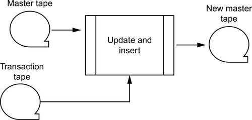
SQL-99 added a single statement to mimic a common magnetic tape file system “merge and insert” procedure. The simplest business logic, in a pseudo-code is like this.
FOR EACH row IN the Transactions table
DO IF working row NOT IN Master table
 THEN INSERT working row INTO the Master table;
 ELSE UPDATE Master table
SET Master table columns to the Transactions table values
 WHERE they meet a matching criteria;
 END IF;
END FOR;
In the 1950s, we would sort the transaction tape(s) and Master tapes on the same key, read each one looking for a match, and then perform whatever logic is needed. In its simplest form, the MERGE statement looks like this (Figure 15.1):
MERGE INTO < table name > [AS [< correlation name >]]
USING < table reference > ON < search condition >
{WHEN [NOT] MATCHED [AND < search condition >]
 THEN < modification operation >} ...
[ELSE IGNORE];
You will notice that use of a correlation name in the MERGE INTO clause is in complete violation of the principle that a correlation name effectively creates a temporary table. There are several other places where SQL:2003 destroyed the original SQL language model, but you do not have to write irregular syntax in all cases.
After a row is MATCHED (or not) to the target table, you can add more < search condition>s in the WHEN clauses in the Standards. Some of the lesser SQLs do not allow extra < search condition>s, so be careful. You can often work around this limitation with logic in the ON, WHERE clauses and CASE expressions.
The < modification operation > clause can include insertion, update, or delete operations that follow the same rules as those single statements. This can hide complex programming logic in a single statement. But the NOT MATCHED indicates the operation to be performed on the rows where the ON search condition is FALSE or UNKNOWN. Only INSERT or signal-statement to raise an exception can be specified after THEN.
Let’s assume that that we have a table of Personnel salary_amt changes at the branch office in a staging table called Personnel_Changes. Here is a MERGE statement, which will take the contents of the Personnel_Changes table and merge them with the Personnel table. Both of them use the emp_nbr as the key. Here is a typical, but very simple use of MERGE INTO.
MERGE INTO Personnel
USING (SELECT emp_nbr, salary_amt, bonus_amt, commission_amt
FROM Personnel_Changes) AS C
 ON Personnel.emp_nbr = C.emp_nbr
WHEN MATCHED
THEN UPDATE
SET (Personnel.salary_amt, Personnel.bonus_amt,  Personnel.commission_amt)
 = (C.salary_amt, C.bonus_amt, C.commission_amt)
WHEN NOT MATCHED
THEN INSERT
(emp_nbr, salary_amt, bonus_amt, commission_amt)
VALUES (C.emp_nbr, C.salary_amt, C.bonus_amt, C.commission_amt);
If you think about it for a minute, if there is a match, then all you can do is UPDATE the row. If there is no match, then all you can do is INSERT the new row.
Consider a fancier version of the second clause, and an employee type that determines the compensation pattern.
WHEN MATCHED AND c.emp_type = 'sales'
THEN UPDATE
SET (Personnel.salary_amt, Personnel.bonus_amt,  Personnel.commission_amt)
 = (C.salary_amt, C.bonus_amt, C.commission_amt)
WHEN MATCHED AND c.emp_type = 'executive'
THEN UPDATE
SET (Personnel.salary_amt, Personnel.bonus_amt,  Personnel.commission_amt)
= (C.salary_amt, C.bonus_amt, 0.00)
WHEN MATCHED AND c.emp_type = 'office'
THEN UPDATE
SET (Personnel.salary_amt, Personnel.bonus_amt,  Personnel.commission_amt)
 = (C.salary_amt, 0.00, 0.00)
There are proprietary versions of this statement in particular, look for the term “upsert” in the literature. These statements are most often used for adding data to a data warehouse in their product.
Your first thought might be that MERGE is a shorthand for this code skeleton:
BEGIN ATOMIC
UPDATE T1
 SET (a, b, c, ..
= (SELECT a, b, c, ..
FROM T2
 WHERE T1.somekey = T2.somekey),
 WHERE EXISTS
(SELECT *
FROM T2
 WHERE T1.somekey = T2.somekey);
INSERT INTO T1
SELECT *
FROM T2
WHERE NOT EXISTS
(SELECT *
FROM T2
 WHERE T1.somekey = T2.somekey);
END;
But there are some subtle differences. The MERGE is a single statement, so it can be optimized as a whole. The two separate UPDATE and INSERT clauses can be optimized as a single statement. The first pass splits the working set into two buckets, and then each MATCHED/NOT MATCHED bucket is handled by itself. The WHEN [NOT] MATCHED clauses with additional search conditions can be executed in parallel or rearranged on the fly, but they have to effectively perform them in left-to-right order.