Comparison or Theta Operators
Dr. Codd introduced the term “theta operators” in his early papers for what a programmer would have called a comparison predicate or operator. The large number of data types in SQL makes doing comparisons a little harder than in other programming languages; we have to do more casting. Values of one data type have to be promoted to values of the other data type before the comparison can be done. The available data types are implementation- and hardware-dependent so read the manuals for your product.
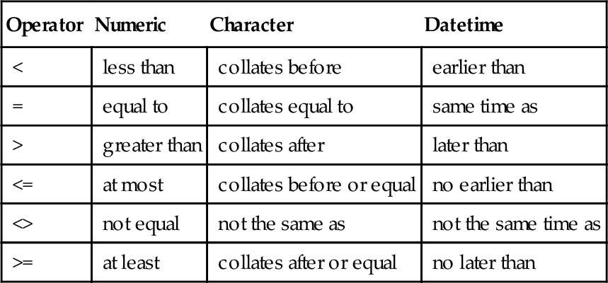
The comparison operators are overloaded and will work for numeric, character, and temporal data types. The symbols and meanings for comparison operators are shown in the table below.
| Operator | Numeric | Character | Datetime |
| < | less than | collates before | earlier than |
| = | equal to | collates equal to | same time as |
| > | greater than | collates after | later than |
| <= | at most | collates before or equal | no earlier than |
| <> | not equal | not the same as | not the same time as |
| >= | at least | collates after or equal | no later than |
You will also see! = or ¬=for “not equal to” in some older SQL implementations. These symbols are borrowed from the C and PL/I programming languages, respectively, and have never been part of standard SQL. It is a bad habit to use them since it destroys portability of your code and makes it harder to read.
The comparison operators will return a logical value of TRUE, FALSE, or UNKNOWN. The values TRUE and FALSE follow the usual rules and UNKNOWN is always returned when one or both of the operands is a NULL. Please pay attention to Section 17.3 on the new IS [NOT] DISTINCT FROM Operator and look at functions that work with NULLs.
17.1 Converting Data Types
Numeric data types are all mutually comparable and mutually assignable. If an assignment would result in a loss of the most significant digits, an exception condition is raised. If least significant digits are lost, the implementation defines what rounding or truncating occurs and does not report an exception condition. Most often, one value is converted to the same data type as the other and then the comparison is done in the usual way. The chosen data type is the “higher” of the two, using the following ordering: SMALLINT, INTEGER, BIGINT, DECIMAL, NUMERIC, REAL, FLOAT, DOUBLE PRECISION.
Floating-point hardware will often affect comparisons for REAL, FLOAT, and DOUBLE PRECISION numbers. There is no good way to avoid this, since it is not always reasonable to use DECIMAL or NUMERIC in their place. A host language will probably use the same floating-point hardware, so at least errors will be constant across the application.
CHARACTER (or CHAR) and CHARACTER VARYING (or VARCHAR) data types are comparable if and only if they are taken from the same character repertoire. This means that ASCII characters cannot be compared with graphics characters, English cannot be compared to Arabic, and so on. In most implementations this is not a problem, because the database usually has only one repertoire.
The comparison takes the shorter of the two strings and pads it with spaces. The strings are compared position by position from left to right, using the collating sequence for the repertoire—ASCII or EBCDIC in most cases.
Temporal (or < datetime >, as they are called in the standard) data types are mutually assignable only if the source and target of the assignment have the same < datetime > fields. That is, you cannot compare a date and a time. The CAST() operator can do explicit type conversions before you do a comparison.
Here is a table of the valid combinations of source (rows in the table) and target (columns) data types in Standard SQL. Y (“yes”) means that the combination is syntactically valid without restriction; M (“maybe”) indicates that the combination is valid subject to other syntax rules; and N (“no”) indicates that the combination is not valid.
| EN | AN | VC | FC | VB | FB | D | T | TS | YM | DT | |
| EN | Y | Y | Y | Y | N | N | N | N | N | N | M |
| AN | Y | Y | Y | Y | N | N | N | N | N | N | N |
| C | Y | Y | M | M | Y | Y | Y | Y | Y | Y | Y |
| B | N | N | Y | Y | Y | Y | N | N | N | N | N |
| D | N | N | Y | Y | N | N | Y | N | Y | N | N |
| T | N | N | Y | Y | N | N | N | Y | Y | N | N |
| TS | N | N | Y | Y | N | N | Y | Y | Y | N | N |
| YM | M | N | Y | Y | N | N | N | N | N | Y | N |
| DT | M | N | Y | Y | N | N | N | N | N | N | Y |
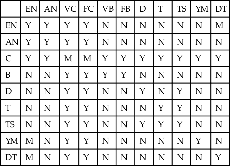
Where:
AN = Approximate Numeric
C = Character (Fixed- or Variable-length)
FC = Fixed-length Character
VC = Variable-length Character
B = Bit String (Fixed- or Variable-length)
FB = Fixed-length Bit String
VB = Variable-length Bit String
D = Date
T = Time
TS = Timestamp
YM = Year-Month Interval
DT = Day-Time Interval
17.1.1 Date Display Formats
SQL is silent about formatting data for display, as it should be. Dates have many different national formats and you will find many vendor extensions that allow the user to format temporal data into strings and to input dates in various display formats. The only subset of the ISO-8601 formats used in Standard SQL is “yyyy-mm-dd hh:mm:ss.sssss”. The year field is between “0001” and “9999”, months and days follow the Common Era Calendar. Hours are between “00” and “23”; minutes are between “00” and “59”; seconds are between “00” and” 59.999..” with the decimal precision being defined by implementation. The FIPS (Federal Information Processing Standards) requires at least 5 decimal places and most modern hard will provide nanosecond accuracy.
17.1.2 Other Display Formats
Character and exact numeric data types are usually displayed as you would expect. Today this means Unicode rules. Approximate numeric data might be shown in decimal or exponential formats. This is implementation defined. However, the Standard defines an approximate numeric literal as:
< approximate numeric literal > ::= < mantissa > E < exponent >
< mantissa > ::= < exact numeric literal >
< exponent > ::= < signed integer >
But some host languages do not require a < mantissa > and some allow a lowercase ‘e’ for the separator. SQL requires a leading zero where other languages might not.
17.2 Row Comparisons in SQL
Standard SQL generalized the theta operators so they would work on row expressions and not just on scalars. This is not a popular feature yet, but it is very handy for situations where a key is made from more than one column, and so forth. This makes SQL more orthogonal and it has an intuitive feel to it. Take three row constants:
B = (10, NULL, 30, 40);
C = (10, NULL, 30, 100);
It seems reasonable to define a row comparison as valid only when the data types of each corresponding column in the rows are union-compatible. If not, the operation is an error and should report a warning. It also seems reasonable to define the results of the comparison to the AND-ed results of each corresponding column using the same operator. That is, (A = B) becomes:
((10, 20, 30, 40) = (10, NULL, 30, 40));
becomes:
((10 = 10) AND (20 = NULL) AND (30 = 30) AND (40 = 40))
becomes:
(TRUE AND UNKNOWN AND TRUE AND TRUE);
becomes:
This seems to be reasonable and conforms to the idea that a NULL is a missing value that we expect to resolve at a future date, so we cannot draw a conclusion about this comparison just yet. Now consider the comparison (A = C), which becomes:
((10, 20, 30, 40) = (10, NULL, 30, 100));
becomes:
((10 = 10) AND (20 = NULL) AND (30 = 30) AND (40 = 100));
becomes:
(TRUE AND UNKNOWN AND TRUE AND FALSE);
becomes:
There is no way to pick a value from column 2 of row C such that the UNKNOWN result will change to TRUE because the fourth column is always FALSE. This leaves you with a situation that is not very intuitive. The first case can resolve to TRUE or FALSE, but the second case can only go to FALSE.
Standard SQL decided that the theta operators would work as shown in the table below. The expression RX < comp op > RY is shorthand for a row RX compared to a row RY; likewise, RXi means the i-th column in the row RX. The results are still TRUE, FALSE, or UNKNOWN, if there is no error in type matching. The rules favor solid tests for TRUE or FALSE, using UNKNOWN as a last resort.
The idea of these rules is that as you read the rows from left to right, the values in one row are always greater than or less than) those in the other row after some column. This is how it would work if you were alphabetizing words.
The rules are:
1. RX = RY is TRUE if and only if RXi = RYi for all i.
2. RX <> RY is TRUE if and only if RXi <> RYi for some i.
3. RX < RY is TRUE if and only if RXi = RYi for all i < n and RXn < RYn for some n.
4. RX > RY is TRUE if and only if RXi = RYi for all i < n and RXn > RYn for some n.
5. RX < = RY is TRUE if and only if Rx = Ry or Rx < Ry.
6. RX > = RY is TRUE if and only if Rx = Ry or Rx > Ry.
7. RX = RY is FALSE if and only if RX <> RY is TRUE.
8. RX <> RY is FALSE if and only if RX = RY is TRUE.
9. RX < RY is FALSE if and only if RX > = RY is TRUE.
10. RX > RY is FALSE if and only if RX < = RY is TRUE.
11. RX < = RY is FALSE if and only if RX > RY is TRUE.
12. 17. RX > = RY is FALSE if and only if RX < RY is TRUE.
13. RX < comp op > RY is UNKNOWN if and only if RX < comp op > RY is neither TRUE nor FALSE.
The negations are defined so that the NOT operator will still have its usual properties. Notice that a NULL in a row will give an UNKNOWN result in a comparison. Consider this expression:
(a, b, c) < (x, y, z)
which becomes
OR ((a = x) AND (b < y))
OR ((a = x) AND (b = y) AND (c < z)))
The standard allows a single-row expression of any sort, including a single-row subquery, on either side of a comparison. Likewise, the BETWEEN predicate can use row expressions in any position in Standard SQL.
17.3 IS [NOT] DISTINCT FROM Operator
The SQL 2003 Standards added a verbose but useful theta operator. SQL has two kinds of comparisons, or equivalence classes; equality and grouping.
Equality treats NULLs as incomparable and gets us into the three valued logic that returns {TRUE, FALSE, UNKNOWN}.
Grouping treats NULLs as equal values and gets us into the usual two valued logic that returns {TRUE, FALSE}. This is why a GROUP BY puts all the NULLs in one group and you get that behavior in other places.
The theta operators we have discussed so far are based on the equality model, so if you wanted a comparison that grouped NULLs, you had to write elaborate CASE expressions. Now you can do it in one infix operator for either rows or scalars.
< expression 1 > IS NOT DISTINCT FROM < expression 2 >
is logically equivalent to
AND < expression 2 > IS NOT NULL
AND < expression 1 > = < expression 2 >)
OR (< expression 1 > IS NULL AND < expression 2 > IS NULL)
Thus following the usual pattern for adding NOT into SQL constructs
< expression 1 > IS DISTINCT FROM < expression 2 >
is a shorthand for
NOT (< expression 1 > IS NOT DISTINCT FROM < expression 2 >)
This double negative was because the IS NOT DISTINCT FROM was defined first. I have no idea why.
You will see an attempt to get this functionality with search conditions like:
COALESCE (< expression 1 >, < absurd non-null value >) = COALESCE (< expression 2 >, < absurd non-null value >)
This avoids the problem that if the second parameter, an absurd value, was NULL, then COALESCE will be “NULL = NULL” which will result in UNKNOWN.
17.4 Monadic Operators
A monadic operator returns a logical value. But the problem in SQL is that we have scalar values, row values and table values. These operators are defined for one or more levels.
17.4.1 IS NULL
< null predicate > ::=<row value constructor > IS [NOT] NULL
It is the only way to test to see if an expression is NULL or not, and it has been in SQL-86 and all later versions of the standard. The SQL-92 standard extended it to accept < row value constructor > instead of a single column or a scalar expression.
This extended version will start showing up in implementations when other row expressions are allowed. If all the values in the row R are the NULL value, then R IS NULL is TRUE; otherwise, it is FALSE. If none of the values in R are NULL value, R IS NOT NULL is TRUE; otherwise, it is FALSE. The case where the row is a mix of NULL and non-NULL values is defined by the table below, where Degree means the number of columns in the row expression.
| Degree of R | R IS NULL | R IS NOT NULL | NOT (R IS NULL) | NOT (R IS NOT NULL) |
| Degree = 1 | ||||
| NULL | TRUE | FALSE | FALSE | TRUE |
| Not NULL | FALSE | TRUE | TRUE | FALSE |
| Degree > 1 | ||||
| All NULLs | TRUE | FALSE | FALSE | TRUE |
| Some NULLs | FALSE | FALSE | TRUE | TRUE |
| No NULLs | FALSE | TRUE | TRUE | FALSE |

Note that R IS NOT NULL has the same result as NOT R IS NULL if and only if R is of degree one. This is a break in the usual pattern of predicates with a NOT option in them. Here are some examples:
(1, NULL, 3) IS NULL = FALSE
(1, NULL, 3) IS NOT NULL = FALSE
(NULL, NULL, NULL) IS NULL = TRUE
(NULL, NULL, NULL) IS NOT NULL = FALSE
NOT (1, 2, 3) IS NULL = TRUE
NOT (1, NULL, 3) IS NULL = TRUE
NOT (1, NULL, 3) IS NOT NULL = TRUE
NOT (NULL, NULL, NULL) IS NULL = FALSE
NOT (NULL, NULL, NULL) IS NOT NULL = TRUE
It is important to remember where NULLs can occur. They are more than just a possible value in a column. Aggregate functions on empty sets, OUTER JOINs, arithmetic expressions with NULLs, and so forth all return NULLs. These constructs often show up as columns in VIEWs.
17.4.2 IS [NOT] {TRUE | FALSE | UNKNOWN}
This predicate tests a condition that has the truth-value TRUE, FALSE, or UNKNOWN, and returns TRUE or FALSE. The syntax is:
< Boolean primary > [IS [NOT] < truth value >]
< truth value > ::= TRUE | FALSE | UNKNOWN
< Boolean primary > ::=
< predicate > | < left paren > < search condition > < right paren >
As you would expect, the expression IS NOT < logical value > is the same as NOT (x IS < logical value >), so the predicate can be defined by the table below.
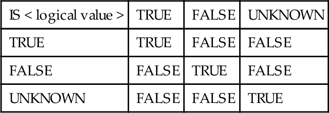
If you are familiar with some of Date’s writings, his MAYBE(x) predicate is not the same as the ANSI (x) IS NOT FALSE predicate, but it is equivalent to the (x) IS UNKNOWN predicate. Date’s predicate excludes the case where all conditions in the predicate are TRUE.
Date points out that it is difficult to ask a conditional question in English. To borrow one of Chris Date’s examples (Date 1990), consider the problem of finding employees who might be programmers born before 1975 January 18 with a salary less than $50,000. The statement of the problem is a bit unclear as to what the “might be” covers—just being a programmer, or all three conditions. Let’s assume that we want some doubt on any of the three conditions. With this predicate, the answer is fairly easy to write:
SELECT *
FROM Personnel
WHERE (job_title = 'Programmer'
AND birth_date < CAST ('1975-01-18' AS DATE)
AND (salary_amt < 50000.00) IS UNKNOWN;
could be expanded in the old SQLs as:
SELECT *
FROM Personnel
WHERE (job_title IS NULL
AND birth_date < CAST ('1975-01-18' AS DATE)
AND salary_amt < 50000.00.00)
 OR (job_title = 'Programmer'
AND birth_date IS NULL
AND salary_amt < 50000.00.00)
 OR (job_title = 'Programmer'
AND birth_date < CAST ('1975-01-18' AS DATE)
AND salary_amt IS NULL)
 OR (job_title IS NULL
AND birth_date IS NULL
AND salary_amt < 50000.00.00)
 OR (job_title IS NULL
AND birth_date < CAST ('1975-01-18' AS DATE)
AND salary_amt IS NULL)
 OR (job_title = 'Programmer'
AND birth_date IS NULL
AND salary_amt IS NULL)
 OR (job_title IS NULL
AND birth_date IS NULL
AND salary_amt IS NULL);
The problem is that every possible combination of NULLs and non-NULLs has to be tested. Since there are three predicates involved, this gives us (3^2) − 1 = 7 combinations to check out (when none of the columns are NULL, we can get a TRUE or FALSE result). The IS NOT UNKNOWN predicate does not have to bother with the combinations, only the final logical value.
17.4.3 IS [NOT] NORMALIZED
< string > IS [NOT] NORMALIZED determines if a Unicode string is one of the four normal forms (D, C, KD and KC). The use of the words “normal form” here are not the same as in a relational context. In the Unicode model, a single character can be built from several other characters. Accent marks can be put on basic Latin letters. Certain combinations of letters can be displayed as ligatures (‘ae’ becomes ‘æ’). Some languages, such as Hangul (Korean) and Vietnamese, build glyphs from concatenating symbols in two dimensions. Some languages have special forms of one letter that are determined by context, such as the terminal lowercase sigma in Greek or accented ‘u’ in Czech. In short, writing is more complex than putting one letter after another.
The Unicode standard defines the order of such constructions in their normal forms. You can still produce the same results with different orderings and sometimes with different combinations of symbols. But it is very handy when you are searching such text to know that it is normalized rather than trying to parse each glyph on the fly. You can find details about normalization and links to free software at www.unicode.org.