VIEWs, Derived, and Other Virtual Tables
Views are also called virtual tables, to distinguish it from temporary and base tables which are persistent. Views and derived tables are the ways of putting a query into a named schema object. By that, I mean these things hold the query code rather than the results of the query. The query is executed and the results are effectively materialized as a table with the view name.
The definition of a VIEW in Standard SQL requires that it acts as if an actual physical table is created when its name is invoked. Whether or not the database system actually materializes the results or uses other mechanisms to get the same effect is implementation defined. The definition of a VIEW is kept in the schema tables to be invoked by name wherever a table could be used. If the VIEW is updatable, then additional rules apply.
The SQL Standard separates administrative (ADMIN) privileges from user (USER) privileges. Table creation is administrative and query execution is a user privilege, so users cannot create their own VIEWs or TEMPORARY TABLEs without having Administrative privileges granted to them.
6.1 VIEWs in Queries
The Standard SQL syntax for the VIEW definition is
CREATE VIEW < table name > AS
[WITH RECURSIVE < table name > (< view column list >)
AS (< query expression >)]
SELECT < view column list > FROM < table name >
< levels clause > ::= CASCADED | LOCAL
We seldom use recursive views. Recursion is expensive, has poor performance and there are better way to do this in the schema design or in the host program. This is basically the same syntax as a recursive query. Here is a VIEW for a table of integers from 1 to 100 done recursively.
CREATE VIEW Nums_1_100 (n) AS
WITH RECURSIVE X (n)
AS (VALUES (1)
UNION ALL
SELECT n+1 FROM Nums_1_100 WHERE n < 100)
SELECT n FROM X;
Now let’s worry about the important stuff.
The < levels clause > option in the WITH CHECK OPTION did not exist in SQL-89 and earlier standards. This clause has no effect on queries, but only on UPDATE, INSERT INTO, and DELETE FROM statements. It is tricky and not well-understood, so we will discuss it in detail later in this chapter.
A VIEW is different from a TEMPORARY TABLE, derived table, and base table. You cannot put constraints on a VIEW, as you can with base and TEMPORARY tables. A VIEW has no existence in the database until it is invoked, while a TEMPORARY TABLE is persistent. A derived table exists only in the scope of the query in which it is created.
The name of the VIEW must be unique within the database schema, like a base table name. The VIEW definition cannot reference itself, since it does not exist yet. Nor can the definition reference only other VIEWs; the nesting of VIEWs must eventually resolve to underlying base tables. This only makes sense; if no base tables were involved, what would you be viewing?
6.2 Updatable and Read-Only VIEWs
Unlike base tables, VIEWs are either updatable or read-only, but not both. INSERT, UPDATE, and DELETE operations are allowed on updatable VIEWs and base tables, subject to any other constraints. INSERT, UPDATE, and DELETE are not allowed on read-only VIEWs, but you can change their base tables, as you would expect.
An updatable VIEW is one that can have each of its rows associated with exactly one row in an underlying base table. When the VIEW is changed, the changes pass through the VIEW to that underlying base table unambiguously. Updatable VIEWs in Standard SQL are defined only for queries that meet these criteria:
(1) They are built on only one table
(2) No GROUP BY clause
(3) No HAVING clause
(4) No aggregate functions
(5) No calculated columns
(6) No UNION, INTERSECT, or EXCEPT
(7) No SELECT DISTINCT clause
(8) Any columns excluded from the VIEW must be NULL-able or have a DEFAULT in the base table, so that a whole row can be constructed for insertion
By implication, the VIEW must also contain a key of the table. In short, we are absolutely sure that each row in the VIEW maps back to one and only one row in the base table.
Some updating is handled by the CASCADE option in the referential integrity constraints on the base tables, not by the VIEW declaration.
The definition of updatability in Standard SQL is actually pretty limited, but very safe. The database system could look at information it has in the referential integrity constraints to widen the set of allowed updatable VIEWs. You will find that some implementations are now doing just that, but it is not common yet. The SQL standard definition of an updatable VIEW is actually a subset of the possible updatable VIEWs, and a very small subset at that! The major advantage of this definition is that it is based on syntax and not semantics. For example, these VIEW skeletons are logically identical:
CREATE VIEW Foo1 -- updatable, has a key!
AS SELECT *
FROM Foobar
WHERE x IN (1,2);
CREATE VIEW Foo2 -- not updatable!
AS SELECT *
FROM Foobar
WHERE x = 1
UNION ALL
SELECT *
FROM Foobar
WHERE x = 2;
But Foo1 is updatable and Foo2 is not. While I know of no formal proof, I suspect that determining if a complex query resolves to an updatable query for allowed sets of data values possible in the table is an NP-complete problem.
Without going into details, here is a list of types of queries that can yield updatable VIEWs, as taken from “VIEW Update Is Practical” (Goodman 1990):
1. Projection from a single table (Standard SQL)
2. Restriction/projection from a single table (Standard SQL)
3. UNION VIEWs
4. Set difference views
5. One-to-one joins
6. One-to-one outer joins
7. One-to-many joins
8. One-to-many outer joins
9. Many-to-many joins
10. Translated and coded columns
It is possible for a user to write INSTEAD OF triggers on VIEWs, which catch the changes and route them to the base tables that make up the VIEW. The database designer has complete control over the way VIEWs are handled. But as Spiderman said, “With great power, comes great responsibility,” and you have to be very careful. I will discuss triggers in detail later.
6.3 Types of VIEWs
The type of SELECT statement and their purpose can classify VIEWs. The strong advantage of a VIEW is that it will produce the correct results when it is invoked, based on the current data. Trying to do the same sort of things with temporary tables or computed columns within a table can be subject to errors and slower to read form disk.
6.3.1 Single-Table Projection and Restriction
In practice, many VIEWs are projections or restrictions on a single base table. This is a common method for obtaining security control by removing rows or columns that a particular group of users is not allowed to see. These VIEWs are usually implemented as in-line macro expansion, since the optimizer can easily fold their code into the final query plan.
6.3.2 Calculated Columns
One common use for a VIEW is to provide summary data across a row. For example, given a table with measurements in metric units, we can construct a VIEW that hides the calculations to convert them into English units.
It is important to be sure that you have no problems with NULL values when constructing a calculated column. For example, given a Personnel table with columns for both salary and commission, you might construct this VIEW:
CREATE VIEW Payroll (emp_nbr, paycheck_amt)
AS
SELECT emp_nbr, (salary + COALESCE(commission), 0.00)
FROM Personnel;
Office workers do not get commissions, so the value of their commission column will be NULL, so we use the COALESCE() function to change the NULLs to zeros.
6.3.3 Translated Columns
Another common use of a VIEW is to translate codes into text or other codes by doing table look ups. This is a special case of a joined VIEW based on a FOREIGN KEY relationship between two tables. For example, an order table might use a part number that we wish to display with a part name on an order entry screen. This is done with a JOIN between the order table and the inventory table, thus:
CREATE VIEW Display_Orders (part_nbr, part_name, . . .)
AS SELECT Orders.part_nbr, Inventory.part_name, . . .
FROM Inventory, Orders
WHERE Inventory.part_nbr = Orders.part_nbr;
Sometimes the original code is kept and sometimes it is dropped from the VIEW. As a general rule, it is a better idea to keep both values even though they are redundant. The redundancy can be used as a check for users, as well as a hook for nested joins in either of the codes.
The idea of JOIN VIEWs to translate codes can be expanded to show more than just one translated column. The result is often a “star” query with one table in the center, joined by FOREIGN KEY relations to many other tables to produce a result that is more readable than the original central table.
Missing values are a problem. If there is no translation for a given code, no row appears in the VIEW, or if an OUTER JOIN was used, a NULL will appear. The programmer should establish a referential integrity constraint to CASCADE changes between the tables to prevent loss of data.
6.3.4 Grouped VIEWs
A grouped VIEW is based on a query with a GROUP BY clause. Since each of the groups may have more than one row in the base from which it was built, these are necessarily read-only VIEWs. Such VIEWs usually have one or more aggregate functions and they are used for reporting purposes. They are also handy for working around weaknesses in SQL. Consider a VIEW that shows the largest sale in each state. The query is straightforward:
CREATE VIEW Big_Sales (state_code, sales_amt_max)
AS SELECT state_code, MAX(sales_amt)
FROM Sales
GROUP BY state_code;
SQL does not require that the grouping column(s) appear in the select clause, but it is a good idea in this case.
These VIEWs are also useful for “flattening out” one-to-many relationships. For example, consider a Personnel table, keyed on the employee number (emp_nbr), and a table of dependents, keyed on a combination of the employee number for each dependent’s parent (emp_nbr) and the dependent’s own serial number (dependent_nbr). The goal is to produce a report of the employees by name with the number of dependents each has.
CREATE VIEW Dependent_Tally1 (emp_nbr, dependent_cnt)
AS SELECT emp_nbr, COUNT(dependent_nbr)
FROM Dependents
GROUP BY emp_nbr;
The report is then simply an OUTER JOIN between this VIEW and the Personnel table. The OUTER JOIN is needed to account for employees without dependents with a NULL value, like this.
SELECT emp_name, dependent_cnt
FROM Personnel AS P1
LEFT OUTER JOIN
DepTally1 AS D1
ON P1.emp_nbr = D1.emp_nbr;
6.3.5 UNION-ed VIEWs
Until recently, a VIEW based on a UNION or UNION ALL operation was read-only because there is no general way to map a change onto just one row in one of the base tables. The UNION operator will remove duplicate rows from the results. Both the UNION and UNION ALL operators hide which table the rows came from. Such VIEWs must use a < view column list >, because the columns in a UNION [ALL] have no names of their own. In theory, a UNION of two disjoint tables, neither of which has duplicate rows in itself should be updatable.
Using the problem given in Section 6.3.4 on grouped VIEWs, this could also be done with a UNION query that would assign a count of zero to employees without dependents, thus:
CREATE VIEW DepTally2 (emp_nbr, dependent_cnt)
AS (SELECT emp_nbr, COUNT(dependent_nbr)
FROM Dependents
GROUP BY emp_nbr)
UNION
(SELECT emp_nbr, 0
FROM Personnel AS P2
WHERE NOT EXISTS (SELECT *
FROM Dependents AS D2
WHERE D2.emp_nbr = P2.emp_nbr));
The report is now a simple INNER JOIN between this VIEW and the Personnel table. The zero value, instead of a NULL value, will account for employees without dependents. The report query looks like this.
SELECT empart_name, dependent_cnt
FROM Personnel, DepTally2
WHERE DepTally2.emp_nbr = Personnel.emp_nbr;
Some of the major databases, such as Oracle and DB2, support inserts, updates, and delete from such views. Under the covers, each partition is a separate table, with a rule for its contents. One of the most common partitioning is temporal, so each partition might be based on a date range. The goal is to improve query performance by allowing parallel access to each partition member.
The trade-off is a heavy overhead under the covers with the UNION-ed VIEW partitioning, however. For example, DB2 attempts to insert any given row into each of the tables underlying the UNION ALL view. It then counts how many tables accepted the row. It has to process the entire view, one table at a time and collect the results.
(1) If exactly one table accepts the row, the insert is accepted.
(2) If no table accepts the row, a “no target” error is raised.
(3) If more than one table accepts the row, then an “ambiguous target” error is raised.
The use of INSTEAD OF triggers gives the user the effect of a single table, but there can still be surprises. Think about three tables; A, B, and C. Table C is disjoint from the other two. Tables A and B overlap. So I can always insert into C and may or may not be able to insert into A and B if I hit overlapping rows.
Going back to my “Y2K Doomsday” consulting days, I ran into a version of such a partition by calendar periods. Their Table C was set up on Fiscal quarters and got leap year wrong because one of the fiscal quarters ended on the last day of February.
Another approach somewhat like this is to declare explicit partitioning rules in the DDL with a proprietary syntax. The system will handle the housekeeping and the user sees only one table. In the Oracle model, the goal is to put parts of the logical table to different physical table spaces. Using standard data types, the Oracle syntax looks like this:
CREATE TABLE Sales
(invoice:nbr INTEGER NOT NULL PRIMARY KEY,
sale_year INTEGER NOT NULL,
sale_month INTEGER NOT NULL,
sale_day INTEGER NOT NULL)
PARTITION BY RANGE (sale_year, sale_month, sale_day)
(PARTITION sales_q1 VALUES LESS THAN (1994, 04, 01) TABLESPACE tsa,
PARTITION sales_q2 VALUES LESS THAN (1994, 07, 01) TABLESPACE tsb,
PARTITION sales_q3 VALUES LESS THAN (1994, 10, 01) TABLESPACE tsc,
PARTITION sales q4 VALUES LESS THAN (1995, 01, 01) TABLESPACE tsd);
Again, this will depend on your product, since this has to do with the physical database and not the logical model.
6.3.6 JOINs in VIEWs
A VIEW whose query expression is a joined table is not usually updatable even in theory.
One of the major purposes of a joined view is to “flatten out” a one-to-many or many-to-many relationship. Such relationships cannot map one row in the VIEW back to one row in the underlying tables on the “many” side of the JOIN. Anything said about a JOIN query could be said about a joined view, so they will not be dealt with here, but in a chapter devoted to a full discussion of joins.
6.3.7 Nested VIEWs
A point that is often missed, even by experienced SQL programmers, is that a VIEW can be built on other VIEWs. The only restrictions are that circular references within the query expressions of the VIEWs are illegal and that a VIEW must ultimately be built on base tables. One problem with nested VIEWs is that different updatable VIEWs can reference the same base table at the same time. If these VIEWs then appear in another VIEW, it becomes hard to determine what has happened when the highest-level VIEW is changed. As an example, consider a table with two keys:
CREATE TABLE Canada
(english INTEGER NOT NULL UNIQUE,
french INTEGER NOT NULL UNIQUE,
eng_word CHAR(30),
fren_word CHAR(30));
INSERT INTO Canada
VALUES (1, 2, 'muffins', 'croissants'),
(2, 1, 'bait', 'escargots'),
CREATE VIEW EnglishWords
AS SELECT english, eng_word
FROM Canada
WHERE eng_word IS NOT NULL;
CREATE VIEW FrenchWords
AS SELECT french, fren_word
FROM Canada
WHERE fren_word IS NOT NULL);
We have now tried the escargots and decided that we wish to change our opinion of them:
UPDATE EnglishWords
SET eng_word = 'appetizer'
WHERE english = 2;
Our French user has just tried haggis and decided to insert a new row for his experience:
UPDATE FrenchWords
SET fren_word = 'd''eaux grasses'
WHERE french = 3;
The row that is created is (NULL, 3, NULL, ‘d’‘eaux grasses’), since there is no way for VIEW FrenchWords to get to the VIEW EnglishWords columns. Likewise, the English VIEW user can construct a row to record his translation, (3, NULL, ‘Haggis,’ NULL). But neither of them can consolidate the two rows into a meaningful piece of data.
To delete a row is also to destroy data; the French-speaker who drops ‘croissants’ from the table also drops ‘muffins’ from VIEW EnglishWords.
6.4 How VIEWs are Handled in the Database Engine
Standard SQL requires a system schema table with the text of the VIEW declarations in it. What would be handy, but is not easily done in all SQL implementations, is to trace the VIEWs down to their base tables by printing out a tree diagram of the nested structure. You should check your user library and see if it has such a utility program (for example, FINDVIEW in the old SPARC library for SQL/DS). There are several ways to handle VIEWs, and systems will often use a mixture of them. The major categories of algorithms are materialization and in-line text expansion.
6.4.1 View Column List
The < view column list > is optional; when it is not given, the VIEW will inherit the column names from the query. The number of column names in the < view column list > has to be the same as the degree of the query expression. If any two columns in the query have the same column name, you must have a < view column list > to resolve the ambiguity. The same column name cannot be specified more than once in the < view column list >.
6.4.2 VIEW Materialization
Materialization means that whenever you use the name of the VIEW, the database engine finds its definition in the schema information tables creates a working table with that name which has the appropriate column names with the appropriate data types. Finally, this new table is filled with the results of the SELECT statement in the body of the VIEW definition.
The decision to materialize a VIEW as an actual physical table is implementation-defined in Standard SQL, but the VIEW must act as if it were a table when accessed for a query. If the VIEW is not updatable, this approach automatically protects the base tables from any improper changes and is guaranteed to be correct. It uses existing internal procedures in the database engine (create table, insert from query), so this is easy for the database to do.
The downside of this approach is that it is not very fast for large VIEWs, uses extra storage space, cannot take advantage of indexes already existing on the base tables, usually cannot create indexes on the new table, and cannot be optimized as easily as other approaches. However, materialization is the best approach for certain VIEWs. A VIEW whose construction has a hidden sort is usually materialized. Queries with SELECT DISTINCT, UNION, GROUP BY, and HAVING clauses are often implemented by sorting to remove duplicate rows or to build groups. As each row of the VIEW is built, it has to be saved to compare it to the other rows, so it makes sense to materialize it.
Some products also give you the option of controlling the materializations yourself. The vendor terms vary. A “snapshot” means materializing a table that also includes a time stamp. A “result set” is a materialized table that is passed to a front end application program for display. Check you particular product.
6.4.3 In-Line Text Expansion
Another approach is to store the text of the CREATE VIEW statement and work it into the parse tree of the SELECT, INSERT, UPDATE, or DELETE statements that use it. This allows the optimizer to blend the VIEW definition into the final query plan. For example, you can create a VIEW based on a particular department, thus:
CREATE VIEW SalesDept (dept_name, city_name, . . .)
AS SELECT 'Sales', city_name, . . .
FROM Departments
WHERE dept_name = 'Sales';
and then use it as a query, thus:
SELECT *
FROM SalesDept
WHERE city_name = 'New York';
The parser expands the VIEW into text (or an intermediate tokenized form) within the FROM clause. The query would become, in effect,
SELECT *
FROM (SELECT 'Sales', city_name, . . .
FROM Departments
WHERE dept_name = 'Sales')
AS SalesDept (dept_name, city_name, . . .)
WHERE city_name = 'New York';
and the query optimizer would then “flatten it out” into
SELECT *
FROM Departments
WHERE (dept_name = 'Sales')
AND (city_name = 'New York'),
Though this sounds like a nice approach, it had problems in early systems where the in-line expansion does not result in proper SQL. An earlier version of DB2 was one such system. To illustrate the problem, imagine that you are given a DB2 table that has a long identification number and some figures in each row. The long identification number is like those 40-digit monsters they give you on a utility bill—they are unique only in the first few characters, but the utility company prints the whole thing out anyway. Your task is to create a report that is grouped according to the first six characters of the long identification number. The immediate naive query uses the SUBSTRING() function:
SELECT SUBSTRING(long_id FROM 1 TO 6), SUM(amt1), SUM(amt2), . . .
 FROM TableA
 GROUP BY id;
This does not work; it is incorrect SQL, since the SELECT and GROUP BY lists do not agree. Other common attempts include GROUP BY SUBSTRING(long_id FROM 1 TO 6), which will fail because you cannot use a function, and GROUP BY 1, which will fail because you can use a column position only in a UNION statement, (column position is now deprecated in Standard SQL) and in the ORDER BY in some products.
The GROUP BY has to have a list of simple column names drawn from the tables of the FROM clause. The next attempt is to build a VIEW:
CREATE VIEW BadTry (short_id, amt1, amt2, . . .)
AS
SELECT SUBSTRING(long_id FROM 1 TO 6), amt1, amt2, . . .
 FROM TableA;
and then do a grouped select on it. This is correct SQL, but it does not work in older versions DB2. The compiler apparently tried to insert the VIEW into the FROM clause, as we have seen, but when it expands it out, the results are the same as those of the incorrect first query attempt with a function call in the GROUP BY clause. The trick was to force DB2 to materialize the VIEW so that you can name the column constructed with the SUBSTRING() function. Anything that causes a sort will do this—the SELECT DISTINCT, UNION, GROUP BY, and HAVING clauses, for example.
Since we know that the short identification number is a key, we can use this VIEW:
CREATE VIEW Shorty (short_id, amt1, amt2, . . .)
AS
SELECT DISTINCT SUBSTRING(long_id FROM 1 TO 6), amt1, amt2, . . .
 FROM TableA;
Then the report query is
SELECT short_id, SUM(amt1), SUM(amt2), . . .
 FROM Shorty
 GROUP BY short_id;
This works fine in DB2. I am indebted to Susan Vombrack of Loral Aerospace for this example. Incidentally, this can be written in Standard SQL as
SELECT *
FROM (SELECT SUBSTRING(long_id FROM 1 TO 6) AS short_id,
SUM(amt1), SUM(amt2), . . .
FROM TableA
GROUP BY long_id)
GROUP BY short_id;
The name on the substring result column in the subquery expression makes it recognizable to the parser.
6.4.4 Pointer Structures
Finally, the system can handle VIEWs with special data structures for the VIEW. This is usually an array of pointers into a base table constructed from the VIEW definition. This is a good way to handle updatable VIEWs in Standard SQL, since the target row in the base table is at the end of a pointer chain in the VIEW structure. Access will be as fast as possible.
The pointer structure approach cannot easily use existing indexes on the base tables. But the pointer structure can be implemented as an index with restrictions. Furthermore, multi-table VIEWs can be constructed as pointer structures that allow direct access to the related rows in the table involved in the JOIN. This is very product-dependent, so you cannot make any general assumptions.
6.4.5 Indexing and Views
Note that VIEWs cannot have their own indexes. However, VIEWs can inherit the indexing on their base tables in some implementations. Like tables, VIEWs have no inherent ordering, but a programmer who knows his particular SQL implementation will often write code that takes advantage of the quirks of that product. In particular, some implementations allow you to use an ORDER BY clause in a VIEW (they are allowed only on cursors in standard SQL). This will force a sort and could materialize the VIEW as a working table. When the SQL engine has to do a sequential read of the entire table, the sort might help or hinder a particular query. There is no way to predict the results.
6.5 WITH CHECK OPTION Clause
If WITH CHECK OPTION is specified, the viewed table has to be updatable. This is actually a fast way to check how your particular SQL implementation handles updatable VIEWs. Try to create a version of the VIEW in question using the WITH CHECK OPTION and see if your product will allow you to create it. The WITH CHECK OPTION was part of the SQL-89 standard, which was extended in Standard SQL by adding an optional < levels clause >. CASCADED is implicit if an explicit LEVEL clause is not given. Consider a VIEW defined as:
CREATE VIEW V1
AS SELECT *
FROM Foobar
WHERE col1 = 'A';
and now UPDATE it with
UPDATE V1 SET col1 = 'B';
The UPDATE will take place without any trouble, but the rows that were previously seen now disappear when we use V1 again. They no longer meet the WHERE clause condition! Likewise, an INSERT INTO statement with VALUES (col1 = ‘B’) would insert just fine, but its rows would never be seen again in this VIEW. VIEWs created this way will always have all the rows that meet the criteria and that can be handy. For example, you can set up a VIEW of rows with a status code of ‘to be done,’ work on them, and change a status code to ‘finished,’ and they will disappear from your view. The important point is that the WHERE clause condition was checked only at the time when the VIEW was invoked.
The WITH CHECK OPTION makes the system check the WHERE clause condition upon insertion or UPDATE. If the new or changed row fails the test, the change is rejected and the VIEW remains the same. Thus, the previous UPDATE statement would get an error message and you could not change certain columns in certain ways. For example, consider a VIEW of salaries under $30,000 defined with a WITH CHECK OPTION to prevent anyone from giving a raise above that ceiling.
The WITH CHECK OPTION clause does not work like a CHECK constraint.
CREATE TABLE Foobar (col_a INTEGER);
CREATE VIEW TestView (col_a)
AS
SELECT col_a FROM Foobar WHERE col_a > 0
WITH CHECK OPTION;
INSERT INTO TestView VALUES (NULL); -- This fails!
CREATE TABLE Foobar_2 (col_a INTEGER CHECK (col_a > 0));
INSERT INTO Foobar_2(col_a)
VALUES (NULL); -- This succeeds!
The WITH CHECK OPTION must be TRUE while the CHECK constraint can be either TRUE or UNKNOWN. Once more, you need to watch out for NULLs.
Standard SQL has introduced an optional < levels clause >, which can be either CASCADED or LOCAL. If no < levels clause > is given, a < levels clause > of CASCADED is implicit. The idea of a CASCADED check is that the system checks all the underlying levels that built the VIEW, as well as the WHERE clause condition in the VIEW itself. If anything causes a row to disappear from the VIEW, the UPDATE is rejected. The idea of a WITH LOCAL check option is that only the local WHERE clause is checked. The underlying VIEWs or tables from which this VIEW is built might also be affected, but we do not test for those effects. Consider two VIEWs built on each other from the salary table:
CREATE VIEW Lowpay
AS SELECT *
FROM Personnel
WHERE salary <= 250;
CREATE VIEW Mediumpay
AS SELECT *
FROM Lowpay
WHERE salary >= 100;
If neither VIEW has a WITH CHECK OPTION, the effect of updating Mediumpay by increasing every salary by $1000 will be passed without any check to Lowpay. Lowpay will pass the changes to the underlying Personnel table. The next time Mediumpay is used, Lowpay will be rebuilt in its own right and Mediumpay rebuilt from it, and all the employees will disappear from Mediumpay.
If only Mediumpay has a WITH CASCADED CHECK OPTION on it, the UPDATE will fail. Mediumpay has no problem with such a large salary, but it would cause a row in Lowpay to disappear, so Mediumpay will reject it. However, if only Mediumpay has a WITH LOCAL CHECK OPTION on it, the UPDATE will succeed. Mediumpay has no problem with such a large salary, so it passes the change along to Lowpay. Lowpay, in turn, passes the change to the Personnel table and the UPDATE occurs. If both VIEWs have a WITH CASCADED CHECK OPTION, the effect is a set of conditions, all of which have to be met. The Personnel table can accept UPDATEs or INSERTs only where the salary is between $100 and $250.
This can become very complex. Consider an example from an ANSI X3H2 paper by Nelson Mattos of IBM (Celko 1993). Let us build a five-layer set of VIEWs, using xx and yy as place holders for CASCADED or LOCAL, on a base table T1 with columns c1, c2, c3, c4, and c5, all set to a value of 10, thus:
CREATE VIEW V1 AS SELECT * FROM T1 WHERE (c1 > 5);
CREATE VIEW V2 AS SELECT * FROM V1 WHERE (c2 > 5)
WITH xx CHECK OPTION;
CREATE VIEW V3 AS SELECT * FROM V2 WHERE (c3 > 5);
CREATE VIEW V4 AS SELECT * FROM V3 WHERE (c4 > 5)
WITH yy CHECK OPTION;
CREATE VIEW V5 AS SELECT * FROM V4 WHERE (c5 > 5);
When we set each one of the columns to zero, we get different results, which can be shown in this chart, where ‘S’ means success and ‘F’ means failure:
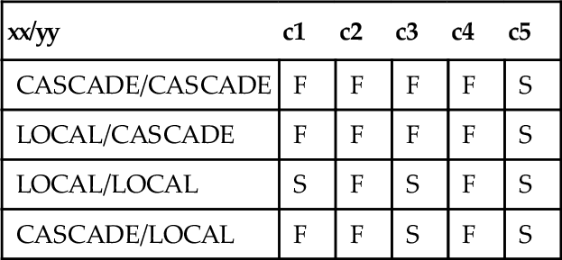
To understand the chart, look at the last line. If xx = CASCADED and yy = LOCAL, updating column c1 to zero via V5 will fail, whereas updating c5 will succeed. Remember that a successful UPDATE means the row(s) disappear from V5.
Follow the action for UPDATE V5 SET c1 = 0; VIEW V5 has no with check options, so the changed rows are immediately sent to V4 without any testing. VIEW V4 does have a WITH LOCAL CHECK OPTION, but column c1 is not involved, so V4 passes the rows to V3. VIEW V3 has no with check options, so the changed rows are immediately sent to V2. VIEW V2 does have a WITH CASCADED CHECK OPTION, so V2 passes the rows to V1 and awaits results. VIEW V1 is built on the original base table and has the condition c1 > 5, which is violated by this UPDATE. VIEW V1 then rejects the UPDATE to the base table, so the rows remain in V5 when it is rebuilt. Now the action for
UPDATE V5 SET c3 = 0;
VIEW V5 has no with check options, so the changed rows are immediately sent to V4, as before. VIEW V4 does have a WITH LOCAL CHECK OPTION, but column c3 is not involved, so V4 passes the rows to V3 without awaiting the results. VIEW V3 is involved with column c3 and has no with check options, so the rows can be changed and passed down to V2 and V1, where they UPDATE the base table. The rows are not seen again when V5 is invoked, because they will fail to get past VIEW V3. The real problem comes with UPDATE statements that change more than one column at a time. For example,
UPDATE V5 SET c1 = 0, c2 = 0, c3 = 0, c4 = 0, c5 = 0;
will fail for all possible combinations of < levels clause > in the example schema.
Standard SQL defines the idea of a set of conditions that are inherited by the levels of nesting. In our sample schema, these implied tests would be added to each VIEW definition:
local/local
V1 = none
V2 = (c2 > 5)
V3 = (c2 > 5)
V4 = (c2 > 5) AND (c4 > 5)
V5 = (c2 > 5) AND (c4 > 5)
cascade/cascade
V1 = none
V2 = (c1 > 5) AND (c2 > 5)
V3 = (c1 > 5) AND (c2 > 5)
V4 = (c1 > 5) AND (c2 > 5) AND (c3 > 5) AND (c4 > 5)
V5 = (c1 > 5) AND (c2 > 5) AND (c3 > 5) AND (c4 > 5)
local/cascade
V1 = none
V2 = (c2 > 5)
V3 = (c2 > 5)
V4 = (c1 > 5) AND (c2 > 5) AND (c4 > 5)
V5 = (c1 > 5) AND (c2 > 5) AND (c4 > 5)
cascade/local
V1 = none
V2 = (c1 > 5) AND (c2 > 5)
V3 = (c1 > 5) AND (c2 > 5)
V4 = (c1 > 5) AND (c2 > 5) AND (c4 > 5)
V5 = (c1 > 5) AND (c2 > 5) AND (c4 > 5)
6.5.1 WITH CHECK OPTION as CHECK() clause
Lothar Flatz, an instructor for Oracle Software Switzerland made the observation that while Oracle cannot put subqueries into CHECK() constraints and triggers would not be possible because of the mutating table problem, you can use a VIEW that has a WITH CHECK OPTION to enforce subquery constraints.
For example, consider a hotel registry that needs to have a rule that you cannot add a guest to a room that another is or will be occupying. Instead of writing the constraint directly, like this:
CREATE TABLE Hotel
(room_nbr INTEGER NOT NULL,
 arrival_date DATE NOT NULL,
 departure_date DATE NOT NULL,
 guest_name CHAR(30) NOT NULL,
 CONSTRAINT schedule_right
 CHECK (H1.arrival_date <= H1.departure_date),
 CONSTRAINT no_overlaps
 CHECK (NOT EXISTS
 (SELECT *
FROM Hotel AS H1, Hotel AS H2
WHERE H1.room_nbr = H2.room_nbr
AND H2.arrival_date < H1.arrival_date
AND H1.arrival_date < H2.departure_date)));
The schedule_right constraint is fine, since it has no subquery, but many products will choke on the no_overlaps constraint. Leaving the no_overlaps constraint off the table, we can construct a VIEW on all the rows and columns of the Hotel base table and add a WHERE clause which will be enforced by the WITH CHECK OPTION.
CREATE VIEW Hotel_V (room_nbr, arrival_date, departure_date, guest_name)
AS SELECT H1.room_nbr, H1.arrival_date, H1.departure_date, H1.guest_name
FROM Hotel AS H1
WHERE NOT EXISTS
(SELECT *
FROM Hotel AS H2
WHERE H1.room_nbr = H2.room_nbr
AND H2.arrival_date < H1.arrival_date
AND H1.arrival_date < H2.departure_date)
AND H1.arrival_date <= H1.departure_date
WITH CHECK OPTION;
For example,
INSERT INTO Hotel_V
VALUES (1, '2006-01-01', '2006-01-03', 'Ron Coe'),
COMMIT;
INSERT INTO Hotel_V
VALUES (1, '2006-01-03', '2006-01-05', 'John Doe'),
will give a WITH CHECK OPTION clause violation on the second INSERT INTO statement, as we wanted.
6.6 Dropping VIEWs
VIEWs, like tables, can be dropped from the schema. The Standard SQL syntax for the statement is:
DROP VIEW < table name > < drop behavior >
< drop behavior > ::= [CASCADE | RESTRICT]
The < drop behavior > clause did not exist in SQL-86, so vendors had different behaviors in their implementation. The usual way of storing VIEWs was in a schema-level table with the VIEW name, the text of the VIEW, and other information. When you dropped a VIEW, the engine usually removed the appropriate row from the schema tables. You found out about dependencies when you tried to use VIEWs built on other VIEWs that no longer existed. Likewise, dropping a base table could cause the same problem when the VIEW was accessed.
The CASCADE option will find all other VIEWs that use the dropped VIEW and remove them also. If RESTRICT is specified, the VIEW cannot be dropped if there is anything that is dependent on it. This implies a structure for the schema tables that is different from just a simple single table.
The bad news is that some older products will let you drop the table(s) from which the view is built, but not drop the view itself.
CREATE TABLE Foobar (col_a INTEGER);
CREATE VIEW TestView
AS SELECT col_a
FROM Foobar;
DROP TABLE Foobar; -- drop the base table
Unless you also cascaded the DROP TABLE statement, the text of the view definition was still in the system. Thus, when you re-use the table and column names, they are resolved at run-time with the view definition.
CREATE TABLE Foobar
(foo_key CHAR(5) NOT NULL PRIMARY KEY,
col_a REAL NOT NULL);
INSERT INTO Foobar VALUES ('Celko', 3.14159);
This is a potential security flaw and a violation of the SQL Standard, but be aware that it exists. Notice that the data type of TestView.col_a changed from INTEGER to REAL along with the new version of the table.
6.7 Materialized Query Tables
DB2 has a feature know as “Materialized Query Table” (MQT) which is based upon the result of a query. MQTs can be used for summary tables and staging tables. You can think of an MQT as a kind of materialized view. Both views and MQTs are defined on the basis of a query. The query on which a view is based is run whenever the view is referenced; however, an MQT actually stores the query results as data, and you can work with the data that is in the MQT instead of the data that is in the underlying tables.
6.7.1 CREATE TABLE
MQTs are created by executing a special form of the CREATE TABLE statement:
CREATE TABLE < table name >
AS
(< select statement >)
DATA INITIALLY DEFERRED
REFRESH [DEFERRED | IMMEDIATE]
[ENABLE | DISABLE] QUERY OPTIMIZATION
MAINTAINED BY [SYSTEM | USER]
A system-maintained MQTs and user-maintained MQTs are the major options. INSERT, UPDATE, and DELETE operations cannot be performed against system-maintained MQTs. These operations are known as “database events” when they are detected by triggers.
REFRESH IMMEDIATE system-maintained MQT is updated automatically, as changes are made to all underlying tables upon which the MQT is based. The REFRESH keyword lets you control how the data in the MQT is to be maintained: REFRESH IMMEDIATE indicates that changes made to underlying tables are cascaded to the MQT as they happen, and REFRESH DEFERRED means that the data in the MQT will be refreshed only when the REFRESH TABLE statement is executed.
User-maintained MQTs allow INSERT, UPDATE, or DELETE operations to be executed against them and can be populated with import and load operations. However, they cannot be populated by executing the REFRESH TABLE statement, nor can they be created with the REFRESH IMMEDIATE option specified. Essentially, a user-defined MQT is a summary table that the DBA is responsible for populating, but one that the DB2 optimizer can utilize to improve query performance. If you do not want the optimizer to utilize an MQT, simply specify the DISABLE QUERY OPTIMIZATION option with the CREATE TABLE statement used to construct the MQT.
6.7.2 REFRESH TABLE Statement
The REFRESH TABLE statement refreshes the data in a materialized query table.
REFRESH TABLE < materialized table name list >
[ [NOT] INCREMENTAL]
[ALLOW [NO | READ | WRITE ] ACCESS]
The INCREMENTAL options allows the user to refresh the whole table or to use the delta in the data since the last refresh. If neither INCREMENTAL nor NOT INCREMENTAL is specified, the system will determine whether incremental processing is possible; if not, full refresh will be performed.
You can specify the accessibility of the table while it is being processed. This is a version of the usual session options in the transaction levels.
ALLOW NO ACCESS = Specifies that no other users can access the table while it is being refreshed.
ALLOW READ ACCESS = Specifies that other users have read-only access to the table while it is being refreshed.
ALLOW WRITE ACCESS = Specifies that other users have read and write access to the table while it is being refreshed.
There are more options that deal with optimization, but this give you the flavor of the statement.