OLAP Aggregation in SQL
Most sql programmers work with OLTP (online transaction processing) databases and write simple, one-level aggregations. This chapter reviews how the usual GROUP BY clause works. The result set is partitioned by the grouping columns, then each group is reduced to a single row. For example, if I group personnel by their departments, I can get the total salaries in each department, but I cannot see the salary of each employee. The employee is at a lower level of aggregation.
25.1 Querying Versus Reporting
Proper queries return tables. A table is a set and all the rows are of the same kind of thing. Reports, also known as OLAP queries, mix unlike things into the same row or the same table. To use the prior example, a row might have the salary of an individual employee in one column, the average salary in his department in a second column, and the total amount of all salaries in the company in a third column in the same row.
A reporting tool can format the data for display, each line on the printout can be different. But an SQL query is required to return something that looks like a table—columns of known data types and rows of a known number of columns. This means that I need to be able to determine the aggregation level of a row in an OLAP query, so I can display it. We need to use NULLs for columns that are “empty” because that level of aggregation does not include a particular column; the row with the average departmental salary would not have an employee name.
Some of this is easier to explain with the actual extensions in SQL.
25.2 GROUPING Operators
OLAP functions add the ROLLUP and CUBE extensions to the GROUP BY clause. The ROLLUP and CUBE are often referred to as super-groups. They can be written in older Standard SQL using GROUP BY and UNION operators.
As expected, NULLs form their own group just as before. However, we now have a GROUPING(< column reference >) function which checks for NULLs that are the results of aggregation over that < column reference > during the execution of a grouped query containing CUBE, ROLLUP, or GROUPING SET, and returns 1 if they were created by the query and a zero otherwise.
SQL:2003 added a multicolumn version that constructs a binary number from the ones and zeros of the columns in the list in an implementation defined exact numeric data type. Here is a recursive definition:
GROUPING (< column ref 1 >, . . ., < column ref n-1 >, < column ref n >)
is equivalent to:
(2 *(< column ref 1 >, . . ., < column ref n-1 >) + GROUPING (< column ref n >))
25.2.1 GROUP BY GROUPING SET
The GROUPING SET(< column list >) is shorthand for a series of UNION-ed queries that are common in reports. For example, to find the total:
SELECT dept_name, CAST(NULL AS CHAR(10)) AS job_title, COUNT(*)
FROM Personnel
GROUP BY dept_name
UNION ALL
SELECT CAST(NULL AS CHAR(8)) AS dept_name, job_title, COUNT(*)
FROM Personnel
GROUP BY job_title;
The above can be rewritten like this:
SELECT dept_name, job_title, COUNT(*)
FROM Personnel
GROUP BY GROUPING SET (dept_name, job_title);
There is a problem with all of the OLAP grouping functions. They will generate NULLs for each dimension at the subtotal levels. How do you tell the difference between a real NULL and a generated NULL? This is a job for the GROUPING() function which returns 0 for NULLs in the original data and 1 for generated NULLs that indicate a subtotal.
SELECT CASE GROUPING(dept_name)
 WHEN 1 THEN 'department total'
 ELSE dept_name END AS dept_name,
 CASE GROUPING(job_title)
 WHEN 1 THEN 'job total'
 ELSE job_title_name END AS job_title
FROM Personnel
GROUP BY GROUPING SETS (dept_name, job_title);
The grouping set concept can be used to define other OLAP groupings.
25.2.2 ROLLUP
A ROLLUP group is an extension to the GROUP BY clause in SQL-99 that produces a result set that contains subtotal rows in addition to the aregular’ grouped rows. Subtotal rows are super-aggregate rows that contain further aggregates whose values are derived by applying the same column functions that were used to obtain the grouped rows. A ROLLUP grouping is a series of grouping sets:
GROUP BY ROLLUP (a, b, c)
is equivalent to:
GROUP BY GROUPING SETS
(a, b, c)
(a, b)
(a)
()
Notice that the (n) elements of the ROLLUP translate to (n + 1) grouping set. Another point to remember is that the order in which the grouping-expression is specified is significant for ROLLUP.
The ROLLUP is basically the classic totals and subtotals report presented as an SQL table.
25.2.3 CUBES
The CUBE super-group is the other SQL-99 extension to the GROUP BY clause that produces a result set that contains all the subtotal rows of a ROLLUP aggregation and, in addition, contains ‘cross-tabulation’ rows. Cross-tabulation rows are additional ‘super-aggregate’ rows. They are, as the name implies, summaries across columns if the data were represented as a spreadsheet. Like ROLLUP, a CUBE group can also be thought of as a series of grouping sets. In the case of a CUBE, all permutations of the cubed grouping-expression are computed along with the grand total. Therefore, the n elements of a CUBE translate to 2n grouping sets:
GROUP BY CUBE (a, b, c)
is equivalent to:
GROUP BY GROUPING SETS
(a, b, c) (a, b) (a, c) (b, c) (a) (b) (c) ()
Notice that the three elements of the CUBE translate to eight grouping sets. Unlike ROLLUP, the order of specification of elements doesn’t matter for CUBE:
CUBE (julian_day, sales_person) is the same as CUBE (sales_person, julian_day).
CUBE is an extension of the ROLLUP function. The CUBE function not only provides the column summaries we saw in ROLLUP but also calculates the row summaries and grand totals for the various dimensions.
25.2.4 OLAP Examples of SQL
The following example illustrates advanced OLAP function used in combination with traditional SQL. In this example, we want to perform a ROLLUP function of sales by region and city:
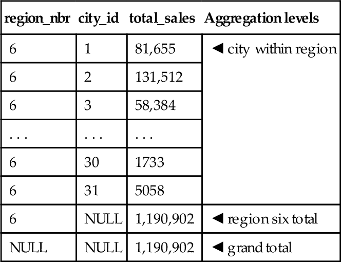
SELECT B.region_nbr, S.city_id, SUM(S.sales_amt) AS total_sales
FROM SalesFacts AS S, MarketLookup AS M
WHERE S.city_id = B.city_id
 AND B.region_nbr = 6
GROUP BY ROLLUP(B.region_nbr, S.city_id);
The resultant set is reduced by explicitly querying region 6. A sample result of the SQL is shown below. The result shows ROLLUP of two groupings (region, city) returning three totals, including region, city, and the grand total. Yearly sales by city and region:
25.3 The Window Clause
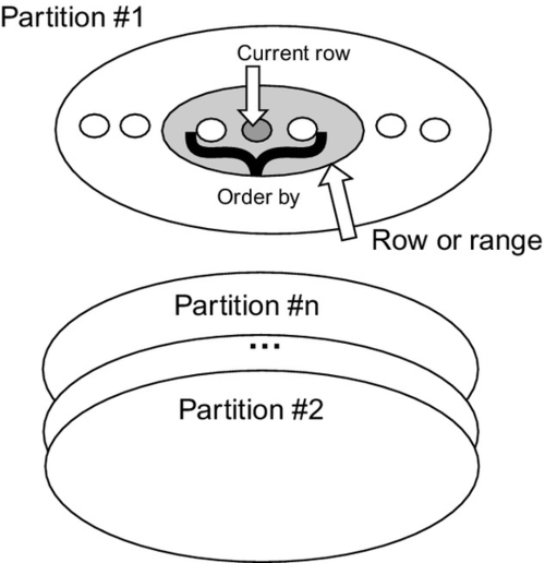
The window clause is also called the OVER() clause informally. The idea is that the table is first broken into partitions with the PARTITION BY subclause. The partitions are then sorted by the ORDER BY clause. An imaginary cursor sits on the current row where the windowed function is invoked. A subset of the rows in the current partition is defined by the number of rows before and after the current row; if there is a < window frame exclusion > option then certain rows are removed from the subset. Finally, the subset is passed to an aggregate or ordinal function to return a scalar value. The window functions follow the rules of any function, but with a different syntax. The window part can be either a < window name > or a < window specification >. The < window specification > gives the details of the window in the OVER() clause and this is how most programmers use it. However, you can define a window and give it a name, then use the name in the OVER() clauses of several statements.
The window works the same way, regardless of the syntax used. The BNF is
< window function >::= < window function type > OVER < window name or specification >
< window function type >::=
 < rank function type > | ROW_NUMBER ()| < aggregate function >
< rank function type >::= RANK() | DENSE_RANK() | PERCENT_RANK() | CUME_DIST()
< window name or specification >::= < window name > | < in-line window specification >
< in-line window specification >::= < window specification >
The window clause has three subclauses: partitioning, ordering, and aggregation grouping or window frame.
25.3.1 PARTITION BY Subclause
A set of column names specifies the partitioning, which is applied to the rows that the preceding FROM, WHERE, GROUP BY, and HAVING clauses produced. If no partitioning is specified, the entire set of rows composes a single partition and the aggregate function applies to the whole set each time. Though the partitioning looks a bit like a GROUP BY, it is not the same thing. A GROUP BY collapses the rows in a partition into a single row. The partitioning within a window, though, simply organizes the rows into groups without collapsing them.
25.3.2 ORDER BY Subclause
The ordering within the window clause is like the ORDER BY clause in a CURSOR. It includes a list of sort keys and indicates whether they should be sorted ascending or descending. The important thing to understand is that ordering is applied within each partition. The other subclauses are optional, but don’t make any sense without an ORDER BY and/or PARTITION BY in the function:
< sort specification list >::= < sort specification > [{,<sort specification >}. . .]
< sort specification >::= < sort key > [< ordering specification >] [< null ordering >]
< sort key >::= < value expression >
< ordering specification >::= ASC | DESC
< null ordering >::= NULLS FIRST | NULLS LAST
It is worth mentioning that the rules for an ORDER BY subclause have changed to be more general than they were in earlier SQL Standards:
1. A sort can now be a < value expression > and is not limited to a simple column in the select list. However, it is still a good idea to use only column names so that you can see the sorting order in the result set.
2. < sort specification > specifies the sort direction for the corresponding sort key. If DESC is not specified in the i-th < sort specification >, then the sort direction for Ki is ascending and the applicable < comp op > is the < less than operator >. Otherwise, the sort direction for Ki is descending and the applicable < comp op > is the < greater than operator >.
3. If < null ordering > is not specified, then an implementation defined < null ordering > is implicit. This was a big issue in earlier SQL Standards because vendors handled NULLs differently. NULLs are considered equal to each other, using the grouping model.
4. If one value is NULL and second value is not NULL, then
4.1 If NULLS FIRST is specified or implied, then first value < comp op > second value is considered to be TRUE.
4.2 If NULLS LAST is specified or implied, then first value < comp op > second value is considered to be FALSE.
4.3 If first value and second value are not NULL and the result of “first value < comp op > second value” is UNKNOWN, then the relative ordering of first value and second value is implementation dependent.
5. Two rows that are not distinct with respect to the < sort specification > are said to be peers of each other. The relative ordering of peers is implementation dependent.
25.3.3 Window Frame Subclause
The tricky one is the window frame. Here is the BNF, but you really need to see code for it to make sense.
< window frame clause >::= < window frame units > < window frame extent >
[< window frame exclusion >]
< window frame units >::= ROWS | RANGE
RANGE works with a single-sort key of a numeric, datetime, or interval data type. It is for data that is a little fuzzy on the edges, if you will. If ROWS is specified, then sort list is made of exact numeric with scale zero.
< window frame extent >::= < window frame start > | < window frame between >
< window frame start >::=
UNBOUNDED PRECEDING | < window frame preceding > | CURRENT ROW
< window frame preceding >::= < unsigned value specification > PRECEDING
If the window starts at UNBOUNDED PRECEDING, then the lower bound is always the first row of the partition; likewise, CURRENT ROW explains itself. The < window frame preceding > is an actual count of preceding rows.
< window frame bound >::= < window frame start > | UNBOUNDED FOLLOWING | < window frame following >
< window frame following >::= < unsigned value specification > FOLLOWING
If the window starts at UNBOUNDED FOLLOWING, then the lower bound is always the last row of the partition; likewise, CURRENT ROW explains itself. The < window frame following > is an actual count of following rows:
< window frame between >::= BETWEEN < window frame bound 1 > AND < window frame bound 2 >
< window frame bound 1 >::= < window frame bound >
< window frame bound 2 >::= < window frame bound >
The current row and its window frame have to stay inside the partition, so the following and preceding limits can effectively change at either end of the frame:
< window frame exclusion >::= EXCLUDE CURRENT ROW | EXCLUDE GROUP
| EXCLUDE TIES | EXCLUDE NO OTHERS
The < window frame exclusion > is not used much or widely implemented. It is also hard to explain. The term “peer” refers to duplicate values.
(1) EXCLUDE CURRENT ROW removes the current row from the window.
(2) EXCLUDE GROUP removes the current row and any peers of the current row.
(3) EXCLUDE TIES removed any rows other than the current row that are peers of the current row.
(4) EXCLUDE NO OTHERS makes sure that no additional rows are removed (Figure 25.1).
25.4 Windowed Aggregate Functions
The regular aggregate functions can take a window clause:
< aggregate function >
OVER ([PARTITION BY < column list >]
[ORDER BY < sort column list >]
[< window frame >])
< aggregate function >::=
 MIN([DISTINCT | ALL] < value exp >) | MAX([DISTINCT | ALL]  < value exp >)
| SUM([DISTINCT | ALL] < value exp >) | AVG([DISTINCT | ALL] < value exp >)
| COUNT([DISTINCT | ALL] [< value exp > | *])
There are no great surprises here. The window that is constructed acts as if it was a group to which the aggregate function is applied.
25.5 Ordinal Functions
The ordinal functions use the window clause but must have an ORDER BY subclause to make sense. They return an ordering of the row within its partition or window frame relative to the rest of the rows in the partition. They have no parameters.
25.5.1 Row Numbering
ROW_NUMBER() uniquely identifies rows with a sequential number based on the position of the row within the window defined by an ordering clause (if one is specified), starting with 1 for the first row and continuing sequentially to the last row in the window. If an ordering clause, ORDER BY, isn’t specified in the window, the row numbers are assigned to the rows in arbitrary order.
25.5.2 RANK() and DENSE_RANK()
RANK() assigns a sequential rank of a row within a window. The RANK() of a row is defined as one plus the number of rows that strictly precede the row. Rows that are not distinct within the ordering of the window are assigned equal ranks. If two or more rows are not distinct with respect to the ordering, then there will be one or more gaps in the sequential rank numbering. That is, the results of RANK() may have gaps in the numbers resulting from duplicate values.
DENSE_RANK() also assigns a sequential rank to a row in a window. However, a row’s DENSE_RANK() is one plus the number of rows preceding it that are distinct with respect to the ordering. Therefore, there will be no gaps in the sequential rank numbering, with ties being assigned the same rank.
25.5.3 PERCENT_RANK() and CUME_DIST
These were added in the SQL:2003 Standard and are defined in terms of earlier constructs. Let < approximate numeric type > 1 be an approximate numeric type with implementation defined precision. PERCENT_RANK() OVER < window specification > is equivalent to:
CASE
WHEN COUNT(*)
OVER (< window specification >
 RANGE BETWEEN UNBOUNDED PRECEDING
 AND UNBOUNDED FOLLOWING) = 1
THEN CAST (0 AS < approximate numeric type >)
ELSE (CAST (RANK ()
 OVER (< window specification >) AS < approximate numeric type>1) - 1)
/ (COUNT (*)
OVER (< window specification>1
RANGE BETWEEN UNBOUNDED PRECEDING
 AND UNBOUNDED FOLLOWING) - 1)
END
Likewise, the cumulative distribution is defined with an < approximate numeric type > with implementation defined precision. CUME_DIST() OVER < window specification > is equivalent to:
(CAST (COUNT (*)
 OVER (< window specification >
 RANGE UNBOUNDED PRECEDING) AS < approximate numeric type >)
 / COUNT(*)
OVER (< window specification>1
 RANGE BETWEEN UNBOUNDED PRECEDING
 AND UNBOUNDED FOLLOWING))
You can also go back and define the other windowed in terms of each other, but it is only a curiosity and has no practical value.
RANK() OVER < window specification > is equivalent to:
(COUNT (*) OVER (< window specification > RANGE UNBOUNDED PRECEDING)
-COUNT (*) OVER (< window specification>RANGE CURRENT ROW) + 1)
DENSE_RANK() OVER (< window specification >) is equivalent to:
COUNT (DISTINCT ROW (< value exp 1 >, . . .,<value exp n >))
OVER (< window specification > RANGE UNBOUNDED PRECEDING)
Where < value exp i > is a sort key in the table.
ROW_NUMBER() OVER WNS is equivalent to:
COUNT (*)
OVER (< window specification > ROWS UNBOUNDED PRECEDING)
25.5.4 Some Examples
The < aggregation grouping > defines a set of rows upon which the aggregate function operates for each row in the partition. Thus, in our example, for each month, you specify the set including it and the two preceding rows:
SELECT SH.region_nbr, SH.sales_month, SH.sales_amt,
 AVG(SH.sales_amt)
 OVER (PARTITION BY SH.region_nbr
 ORDER BY SH.sales_month ASC
 ROWS 2 PRECEDING)
 AS moving_average,
 SUM(SH.sales_amt)
 OVER (PARTITION BY SH.region_nbr
 ORDER BY SH.sales_month ASC
 ROWS BETWEEN UNBOUNDED PRECEDING AND CURRENT ROW)
 AS moving_total
FROM Sales_History AS SH;
Here, “AVG(SH.sales_amt) OVER (PARTITION BY…)” is the first OLAP function. The construct inside the OVER() clause defines the window of data to which the aggregate function, AVG() in this example, is applied.
The window clause defines a partitioned set of rows to which the aggregate function is applied. The window clause says to take Sales_History table and then apply the following operations to it.
1. Partition the sales history by region.
2. Order the data by month within each region.
3. Group each row with the two preceding rows in the same region.
4. Compute the windowed average on each grouping.
The database engine is not required to perform the steps in the order described here, but has to produce the same result set as if they had been carried out.
The second windowed function is a cumulative total to date for each region. It is a very column query pattern.
There are two main types of aggregation groups: physical and logical. In physical grouping, you count a specified number of rows that are before or after the current row. The Sales_History example used physical grouping. In logical grouping, you include all the data in a certain interval, defined in terms of a quantity that can be added to, or subtracted from, the current sort key. For instance, you create the same group whether you define it as the current month’s row plus:
(1) The two preceding rows as defined by the ORDER BY clause.
(2) Any row containing a month no less than 2 months earlier.
Physical grouping works well for contiguous data and programmers who think in terms of sequential files. Physical grouping works for a larger variety of data types than logical grouping, because it does not require operations on values.
Logical grouping works better for data that has gaps or irregularities in the ordering and for programmers who think in SQL predicates. Logical grouping works only if you can do arithmetic on the values (such as numeric quantities and dates).
You will find another query pattern used with these functions. The function invocations need to get names to be referenced, so they are put into a derived table which is encased in a containing query.
SELECT X.*
FROM (SELECT < window function 1 > AS W1,
< window function 2 > AS W2,
..
< window function n > AS Wn
FROM ..
[WHERE ..]
 ) AS X
[WHERE..]
[GROUP BY ..];
Using the SELECT * in the containing query is a handy way to save repeating a select clause list over and over.
25.6 Vendor Extensions
You will find that vendors have added their own proprietary windowed functions to their products. While there is no good way to predict what they will do, there are two sets of common extensions. As a programming exercise, I suggest you try to write them in Standard SQL windowed functions so you can translate dialect SQL if you need to do so.
25.6.1 LEAD and LAG Functions
LEAD and LAG functions are nonstandard shorthands you will find in Oracle other SQL products. Rather than compute an aggregate value, they jump ahead or behind the current row and use that value in an expression. They take three arguments and an OVER() clause. The general syntax is shown below:
[LEAD | LAG] (< expr >, < offset >, < default >) OVER (< window specification >)
< expr > is the expression to compute from the leading or lagging row.
< offset > is the position of the leading or lagging row relative to the current row; it has to be a positive integer which defaults to 1.
< default > is the value to return if the < offset > points to a row outside the partition range. Here is a simple example:
SELECT dept_nbr, emp_id, sal_amt,
 LEAD(sal, 1, 0)
 OVER (PARTITION BY dept_nbr
 ORDER BY sal DESC NULLS LAST)AS lead_sal_amt,
 LAG (sal, 1, 0)
 OVER (PARTITION BY dept_nbr
 ORDER BY sal DESC NULLS LAST) AS lag_sal_amt
FROM Personnel;
Results
| dept_nbr | emp_id | sal_amt | lead_sal_amt | lag_sal_amt |
| 10 | 7839 | 5000 | 2450 | 0 |
| 10 | 7782 | 2450 | 1300 | 5000 |
| 10 | 7934 | 1300 | 0 | 2450 |
| 20 | 7788 | 3000 | 3000 | 0 |
| 20 | 7902 | 3000 | 2975 | 3000 |
| 20 | 7566 | 2975 | 1100 | 3000 |
| 20 | 7876 | 1100 | 800 | 2975 |
| 20 | 7369 | 800 | 0 | 1100 |
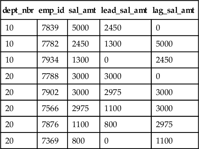
Look at employee 7782, whose current salary is $2450.00. Looking at the salaries, we see that the first salary greater than his is $5000.00 and the first salary less his is $1300.00. Look at employee 7934 whose current salary of $1300.00 puts him at the bottom of the company pay scale; his lead_salary_amt is defaulted to zero.
25.6.1.1 Example with Gaps
Given a sequence of data values, we often miss something. The classic example is reading a meter and getting a gap in the sequence. A common way to handle such missing is to assume that the missing value is the same as the prior known value. For example, every reading we score a foobar on the scale {‘Alpha,’ ‘Beta,’ Gamma’} or post a NULL if we could not get a reading.
CREATE TABLE Foobars
(reading_seq INTEGER NOT NULL PRIMARY KEY,
foo_score CHAR(6)
 CHECK (foo_score IN ('Alpha', 'Beta', Gamma'))
);
INSERT INTO Foobars
VALUES
(1, 'Alpha'),
(2, 'Alpha'),
(3, NULL),
(4, NULL),
(5, NULL),
(6, 'Beta'),
(7, NULL),
(8, 'Beta'),
(9, 'Gamma'),
What we want to do when we have a NULL is assume that we can use the last known value. But a simple LAG() or LEAD() will not work. We have no idea when we had a value. The trick is to use CTEs to get rid of NULLs, then look for ranges in the sequence:
WITH Known_Foo_Scores (reading_seq, foo_score)
AS
(SELECT reading_seq, foo_score
 FROM Foobars
WHERE foo_score IS NOT NULL),
Known_Reading_Pairs (reading_seq, foo_score, prior_reading_seq, prior_foo_score)
AS
(SELECT reading_seq, foo_score,
 LAG(reading_seq) OVER (ORDER BY reading_seq),
 LAG(foo_score) OVER (ORDER BY reading_seq)
 FROM Known_Foo_Scores)
SELECT DISTINCT F.foo_id,
 COALESCE (F.foo_score, X2.prior_foo_score)
FROM Known_Reading_Pairs AS X2, Foobars AS F
WHERE F.foo_id BETWEEN X2.prior_foo_id AND X2.foo_id;
25.6.2 FIRST and LAST Functions
FIRST and LAST functions are nonstandard shorthands you will find in SQL products in various forms. Rather than compute an aggregate value, they sort a partition on one set of columns, then return an expression from the first or last row of that sort. The expression usually has nothing to do with the sorting columns. This is a bit like the joke about the British Sargent-Major ordering the troops to line up alphabetically by height. The general syntax is
[FIRST | LAST](< expr >) OVER (< window specification >)
Using the imaginary Personnel table again:
SELECT emp_id, dept_nbr, hire_date,
 FIRST(hire_date)
OVER (PARTITION BY dept_nbr
ORDER BY emp_id)
 AS first_hire_by_dept
FROM Personnel;
The results get the hire date for the employee who has the lowest employee id in each department.
| emp_id | dept_nbr | hire_date | first_hire_by_dept | |
| 7369 | 20 | '2017-01-01' | '2017-01-01' | |
| 7566 | 20 | '2017-01-02' | '2017-01-01' | |
| 7902 | 20 | '2017-01-02' | '2017-01-01' | |
| 7788 | 20 | '2017-01-04' | '2017-01-01' | |
| 7876 | 20 | '2017-01-07' | '2017-01-01' | |
| 7499 | 30 | '2017-01-27' | '2017-01-27' | |
| 7521 | 30 | '2017-01-09' | '2017-01-27' | |
| 7844 | 30 | '2017-01-17' | '2017-01-27' | |
| 7654 | 30 | '2017-01-18' | '2017-01-27' | |
| 7900 | 30 | '2017-01-20' | '2017-01-27' |
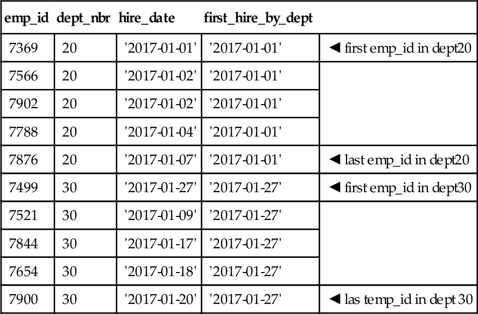
If we had used LAST() instead, the two chosen rows would have been
(7876, 20, ‘2017-01-07,’ ‘2017-01-01’)
(7900, 30, ‘2017-01-20,’ ‘2017-01-27’)
The Oracle extensions FIRST_VALUE and LAST_VALUE are even stranger. They allow other ordinal and aggregate functions to be applied to the retrieved values. If you want to use them, I suggest that you look product specific references and examples.
You can do these with Standard SQL and a little work. The skeleton:
WITH First_Last_Query
AS
(SELECT emp_id, dept_nbr,
ROW_NUMBER()
OVER (PARTITION BY dept_nbr
ORDER BY emp_id ASC) AS asc_order,
ROW_NUMBER()
OVER (PARTITION BY dept_nbr
ORDER BY emp_id DESC) AS desc_order
 FROM Personnel)
SELECT A.emp_id, A.dept_nbr,
 OA.hire_date AS first_value,
 OD.hire_date AS last_value
FROM First_Last_Query AS A,
 First_Last_Query AS OA,
 First_Last_Query AS OD
WHERE OD.desc_order = 1
 AND OA.asc_order = 1;
25.7 A Bit of History
IBM and Oracle jointly proposed these extensions in early 1999 and thanks to ANSI’s uncommonly rapid (and praiseworthy) actions, they are part of the SQL-99 Standard. IBM implemented portions of the specifications in DB2 UDB 6.2, which was commercially available in some forms as early as mid-1999. Oracle 8i version 2 and DB2 UDB 7.1, both released in late 1999, contain beefed-up implementations.
Other vendors contributed, including database tool vendors Brio, MicroStrategy, and Cognos and database vendor Informix, among others. A team lead by Dr. Hamid Pirahesh of IBM’s Almaden Research Laboratory played a particularly important role. After his team had researched the subject for about a year and come up with an approach to extending SQL in this area, he called Oracle. The companies then learned that each had independently done some significant work. With Andy Witkowski playing a pivotal role at Oracle, the two companies hammered out a joint standards proposal in about 2 months. Red Brick was actually the first product to implement this functionality before the standard, but in a less complete form. You can find details in the ANSI document Introduction to OLAP Functions by Fred Zemke, Krishna Kulkarni, Andy Witkowski, and Bob Lyle.