Partitioning and Aggregating Data in Queries
This chapter is concerned with how to break the data in SQL into meaningful subsets that can then be presented to the user or passed along for further reduction.
31.1 Coverings and Partitions
We need to define some basic set operations. A covering is a collection of subsets, drawn from a set, whose union is the original set. A partition is a covering whose subsets do not intersect each other. Cutting up a pizza is a partitioning; smothering it in two layers of pepperoni slices is a covering.
Partitions are the basis for most reports. The property that makes partitions useful for reports is aggregation: the whole is the sum of its parts. For example, a company budget is broken into divisions, divisions are broken into departments, and so forth. Each division budget is the sum of its department’s budgets, and the sum of the division budgets is the total for the whole company again. We would not be sure what to do if a department belonged to two different divisions because that would be a covering and not a partition.
31.1.1 Partitioning by Ranges
A common problem in data processing is classifying things by the way they fall into a range on a numeric or alphabetic scale. The best approach to translating a code into a value when ranges are involved is to set up a table with the high and the low values for each translated value in it. This was covered in the section on auxiliary tables in more detail, but here is a quick review.
Any missing values will easily be detected and the table can be validated for completeness. For example, we could create a table of ZIP code ranges and two-character state_code abbreviation codes like this:
CREATE TABLE State_Zip
(state_code CHAR(2) NOT NULL PRIMARY KEY,
low_zip CHAR(5) NOT NULL UNIQUE,
high_zip CHAR(5) NOT NULL UNIQUE,
CONSTRAINT zip_order_okay CHECK(low_zip <= high_zip),
. . . );
Here is a query that looks up the city_name customer_type and state_code code from the zip code in the Addressbook table to complete a mailing label with a simple JOIN that looks like this:
SELECT A1.customer_type, A1.street_address, SZ.city_name, SZ.state_code, A1.zip
FROM State_Zip AS SZ, Addressbook AS A1
WHERE A1.zip BETWEEN SZ.low_zip AND SZ.high_zip;
You need to be careful with this predicate. If one of the three columns involved has a NULL in it, the BETWEEN predicate becomes UNKNOWN and will not be recognized by the WHERE clause. If you design the table of range values with the high value in one row equal to or greater than the low value in another row, both of those rows will be returned when the test value falls on the overlap.
If you know that you have a partitioning in the range value tables, you can write a query in SQL that will let you use a table with only the high value and the translation code. The grading system table would have (100%, ‘A’), (89%, ‘B’), (79%, ‘C’), (69%, ‘D’), and (59%, ‘F’) as its rows. Likewise, a table of the state_code code and the highest ZIP code in that state_code could do the same job as the BETWEEN predicate in the previous query.
CREATE TABLE State_Zip2
(high_zip CHAR(5) NOT NULL,
state_code CHAR(2) NOT NULL,
PRIMARY KEY (high_zip, state_code));
We want to write a query to give us the greatest lower bound or least upper bound on those values. The greatest lower bound (glb) operator finds the largest number in one column that is less than or equal to the target value in the other column. The least upper bound (lub) operator finds the smallest number greater than or equal to the target number. Unfortunately, this is not a good tradeoff, because the subquery is fairly complex and slow. The “high and low” columns are a better solution in most cases. Here is a second version of the Addressbook query, using only the high_zip column from the State_Zip2 table:
SELECT customer_type, street_address, city_name, state_code, zip
FROM State_Zip2, Addressbook
WHERE state_code =
 (SELECT state_code
FROM State_Zip2
 WHERE high_zip =
(SELECT MIN(high_zip)
FROM State_Zip2
WHERE Address.zip <= State_Zip2.high_zip));
If you want to allow for multiple-row matches by not requiring that the lookup table has unique values, the equality subquery predicate should be converted to an IN() predicate.
31.1.2 Partition by Functions
It is also possible to use a function that will partition the table into subsets that share a particular property. Consider the cases where you have to add a column with the function result to the table because the function is too complex to be reasonably written in SQL.
One common example of this technique is the Soundex function, which is often a vendor extension; the Soundex family assigns codes to names that are phonetically alike. The complex calculations in engineering and scientific databases that involve functions that SQL does not have are another example of this technique.
SQL was never meant to be a computational language. However, many vendors allow a query to access functions in the libraries of other programming languages. You must know what the cost in execution time for your product is before doing this. One version of SQL uses a threaded-code approach to carry parameters over to the other language’s libraries and return the results on each row—the execution time is horrible. Some versions of SQL can compile and link another language’s library into the SQL.
Although this is a generalization, the safest technique is to unload the parameter values to a file in a standard format that can be read by the other language. Then use that file in a program to find the function results and create INSERT INTO statements that will load a table in the database with the parameters and the results. You can then use this working table to load the result column in the original table.
31.1.3 Partition by Sequential Order
We are looking for patterns over a history that has a sequential ordering to it. This ordering could be temporal or via a sequence numbering. For example, given a payment history we want to break it into groupings of behavior, say whether or not the payments were on time or late.
CREATE TABLE Payment_History
(payment_nbr INTEGER NOT NULL PRIMARY KEY,
on_time_flg CHAR(1) DEFAULT 'Y' NOT NULL
 CHECK(on_time_flg IN ('Y', 'N')));
INSERT INTO Payment_History
VALUES (1006, 'Y'),
 (1005, 'Y'),
 (1004, 'N'),
 (1003, 'Y'),
 (1002, 'Y'),
 (1001, 'Y'),
 (1000, 'N'),
The results that we want assign a grouping number to each run of on-time/late payments, thus.
Here is a solution from Hugo Kornelis that depends on the payments always being numbered consecutively.
SELECT (SELECT COUNT(*)
FROM Payment_History AS H2,
 Payment_History AS H3
WHERE H3.payment_nbr = H2.payment_nbr + 1
 AND H3.on_time_flg <> H2.on_time_flg
 AND H2.payment_nbr >= H1.payment_nbr) + 1 AS grp,
payment_nbr, on_time_flg
FROM Payment_History AS H1;
This is very useful when looking for patterns in a history. A more complex version of the same problem would involve more than two categories. Consider a table with a sequential numbering and a list of products that have been received.
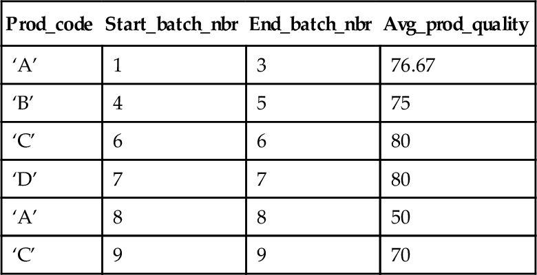
What we want is the average quality score value for a sequential grouping of the same Product. For example, I need an average of Entries 1, 2, and 3 because this is the first grouping of the same product type, but not want that average to include entry #8, which is also Product A, but in a different “group.”
CREATE TABLE Product_Tests
(batch_nbr INTEGER NOT NULL PRIMARY KEY,
prod_code CHAR(1) NOT NULL,
prod_quality DECIMAL(8,4) NOT NULL);
INSERT INTO Product_Tests (batch_nbr, prod_code, prod_quality)
VALUES (1, 'A', 80),
 (2, 'A', 70),
 (3, 'A', 80),
 (4, 'B', 60),
 (5, 'B', 90),
 (6, 'C', 80),
 (7, 'D', 80),
 (8, 'A', 50),
 (9, 'C', 70);
The query then becomes:
SELECT X.prod_code, MIN(X.batch_nbr) AS start_batch_nbr, end_batch_nbr,
 AVG(B4.prod_quality) AS avg_prod_quality
FROM (SELECT B1.prod_code, B1.batch_nbr,
 MAX(B2.batch_nbr) AS end_batch_nbr
FROM Product_Tests AS B1, Product_Tests AS B2
 WHERE B1.batch_nbr <= B2.batch_nbr
 AND B1.prod_code = B2.prod_code
 AND B1.prod_code
 = ALL (SELECT prod_code
 FROM Product_Tests AS B3
WHERE B3.batch_nbr BETWEEN B1.batch_nbr
 AND B2.batch_nbr)
GROUP BY B1.prod_code, B1.batch_nbr) AS X
INNER JOIN
Product_Tests AS B4 -- join to get the quality measurements
ON B4.batch_nbr BETWEEN X.batch_nbr AND X.end_batch_nbr
GROUP BY X.prod_code, X.end_batch_nbr ;
31.2 Advanced Grouping, Windowed Aggregation, and OLAP in SQL
Most SQL programmers work with OLTP (Online Transaction Processing) databases and have had no exposure to Online Analytic Processing (OLAP) and data warehousing. OLAP is concerned with summarizing and reporting data, so the schema designs and common operations are very different from the usual SQL queries.
As a gross generalization, everything you knew in OLTP is reversed in a data warehouse.
(1) OLTP changes data in short, frequent transactions. A data warehouse is bulk loaded with static data on a schedule. The data remains constant once it is in place.
(2) OLTP databases want to store only the data needed to do its current work. A data warehouse wants all the historical data it can hold. In 2008, Teradata Corporation announced that they had five customers running data warehouses larger than a petabyte. The “Petabyte Power Players” club included eBay, with 5 petabytes of data; Wal-Mart Stores, which has 2.5 petabytes; Bank of America, which is storing 1.5 petabytes; Dell, which has a 1 petabyte data warehouse; an unnamed bank. The definition of a petabyte is 250 = 1,125,899,906,842,624 bytes = 1024 terabytes or roughly 1015 bytes.
(3) OLTP queries tend to be for simple facts. Data warehouse queries tend to be aggregate relationships that are more complex. For example, an OLTP query might ask, “How much chocolate did Joe Celko buy?” while a data warehouse might ask, “What is the correlation between chocolate purchases, geographic location, and wearing tweed?”
(4) OLTP wants to run as fast as possible. A data warehouse is more concerned with the accuracy of computations and it is willing to wait to get an answer to a complex query.
(5) Properly designed OLTP databases are normalized. A data warehouse is usually a Star or Snowflake Schema, which is highly denormalized. The Star Schema is due to Ralph Kimball and you can get more details about it in his books and articles.
The Star Schema is a violation of basic normalization rules. There is a large central fact table. This table contains all the facts about an event that you wish to report on, such as sales, in one place. In an OLTP, the inventory would be in one table, the sale in another table, customers in a third table, and so forth. In the data warehouse, they are all in one huge table.
The dimensions of the values in the fact are in smaller tables that allow you to pick a scale or unit of measurement on that dimension in the fact table. For example, the time dimension for the Sales fact table might be grouped by year, month within year, week within month. Then a weight dimension could give you pounds, kilograms, or stock packaging sizes. A category dimension might classify the stocks by department. And so forth. This lets me ask for my fact aggregated in any granularity of units I wish, and perhaps dropping some of the dimensions.
Until recent changes in SQL, OLAP queries had to be done with special OLAP-centric languages, such as Microsoft’s Multidimensional Expressions (MDX). Be assured that the power of OLAP is not found in the wizards or GUIs presented in the vendor demos. The wizards and GUI are often the glitter that lures the uninformed.
Many aspects of OLAP are already integrated with the relational database engine, itself. This blending of technology blurs the distinction between an RDBMS and OLAP data management technology, effectively challenging the passive role often relegated to relational databases with regard to dimensional data. The more your RDBMS can address the needs of both traditional relational data and dimensional data, and then you can reduce the cost of OLAP-only technology and get more out of your investment in RDBMS technology, skills and resources. But do not confuse what SQL can do for you with a reporting tools or the power of a statistical package, either.
31.2.1 GROUPING Operators
OLAP functions add the ROLLUP and CUBE extensions to the GROUP BY clause. The ROLLUP and CUBE are often referred to as super-groups. They can be written in older Standard SQL using GROUP BY and UNION operators.
As expected, NULLs form their own group just as before. However, we now have a GROUPING (< column reference >) function which checks for NULLs that are the results of aggregation over that < column reference > during the execution of a grouped query containing CUBE, ROLLUP, or GROUPING SET, and returns one if they were created by the query and a zero otherwise.
SQL:2003 added a multicolumn version that constructs a binary number from the ones and zeros of the columns in the list in an implementation defined exact numeric data type. Here is a recursive definition:
GROUPING (< column ref 1 >, …, < column ref n-1 >, < column ref n >)
is equivalent to
(2*(< column ref 1 >, …, < column ref n-1 >) + GROUPING (< column ref n >))
31.2.2 GROUP BY GROUPING SET
The GROUPING SET (< column list >) is short hand in SQL-99 for a series of UNION-ed queries that are common in reports. For example, to find the total
SELECT dept_name, CAST(NULL AS CHAR(10)) AS job_title, COUNT(*)
FROM Personnel
GROUP BY dept_name
UNION ALL
SELECT CAST(NULL AS CHAR(8)) AS dept_name, job_title, COUNT(*)
FROM Personnel
GROUP BY job_title;
The above can be rewritten like this.
SELECT dept_name, job_title, COUNT(*)
FROM Personnel
GROUP BY GROUPING SET (dept_name, job_title);
There is a problem with all of the OLAP grouping functions. They will generate NULLs for each dimension at the subtotal levels. How do you tell the difference between a real NULL and a generated NULL? This is a job for the GROUPING() function which returns 0 for NULLs in the original data and 1 for generated NULLs that indicate a subtotal.
SELECT CASE GROUPING(dept_name)
 WHEN 1 THEN 'department total'
 ELSE dept_name END AS dept_name,
 CASE GROUPING(job_title)
 WHEN 1 THEN 'job total'
 ELSE job_title_name END AS job_title
FROM Personnel
GROUP BY GROUPING SETS (dept_name, job_title);
The grouping set concept can be used to define other OLAP groupings.
31.2.3 ROLLUP
A ROLLUP group is an extension to the GROUP BY clause in SQL-99 that produces a result set that contains subtotal rows in addition to the regular grouped rows. Subtotal rows are super-aggregate rows that contain further aggregates whose values are derived by applying the same column functions that were used to obtain the grouped rows. A ROLLUP grouping is a series of grouping-sets.
GROUP BY ROLLUP (a, b, c)
is equivalent to
GROUP BY GROUPING SETS (a, b, c), (a, b), (a),()
Notice that the (n) elements of the ROLLUP translate to (n + 1) grouping set. Another point to remember is that the order in which the grouping-expression is specified is significant for ROLLUP.
The ROLLUP is basically the classic totals and subtotals report presented as an SQL table.
31.2.4 CUBES
The CUBE super-group is the other SQL-99 extension to the GROUP BY clause that produces a result set that contains all the subtotal rows of a ROLLUP aggregation and, in addition, contains ‘cross-tabulation’ rows. Cross-tabulation rows are additional ‘super-aggregate’ rows. They are, as the name implies, summaries across columns if the data were represented as a spreadsheet. Like ROLLUP, a CUBE group can also be thought of as a series of grouping-sets. In the case of a CUBE, all permutations of the cubed grouping-expression are computed along with the grand total. Therefore, the n elements of a CUBE translate to 2n grouping-sets.
GROUP BY CUBE (a, b, c)
is equivalent to
GROUP BY GROUPING SETS
(a, b, c), (a, b), (a, c), (b, c), (a), (b), (c), ()
Notice that the three elements of the CUBE translate to eight grouping sets. Unlike ROLLUP, the order of specification of elements does not matter for CUBE:
CUBE (julian_day, sales_person) is the same as CUBE (sales_person, julian_day).
CUBE is an extension of the ROLLUP function. The CUBE function not only provides the column summaries that we saw in ROLLUP but also calculates the row summaries and grand totals for the various dimensions.
31.2.5 OLAP Examples of SQL
The following example illustrates the advanced OLAP function used in combination with traditional SQL. In this example, we want to perform a ROLLUP function of sales by region and city.
SELECT B.region_nbr, S.city_id, SUM(S.sales_amt) AS total_sales
FROM SalesFacts AS S, MarketLookup AS M
WHERE EXTRACT (YEAR FROM trans_date) = 2011
 AND S.city_id = B.city_id
 AND B.region_nbr = 6
GROUP BY ROLLUP(B.region_nbr, S.city_id);
The resultant set is reduced by explicitly querying region 6 and the year 1999. A sample result of the SQL is shown below. The result shows ROLLUP of two groupings (region, city) returning three totals, including region, city, and grand total.
31.2.6 The Window Clause
The window clause is also called the OVER() clause informally. The idea is that the table is first broken into partitions with the PARTITION BY subclause. The partitions are then sorted by the ORDER BY clause. An imaginary cursor sits on the current row where the windowed function is invoked. A subset of the rows in the current partition is defined by the number of rows before and after the current row; if there is a < window frame exclusion > option then certain rows are removed from the subset. Finally, the subset is passed to an aggregate or ordinal function to return a scalar value. The window functions are functions that follow the rules of any function, but with a different syntax. The window part can be either a < window name > or a < window specification >. The < window specification > gives the details of the window in the OVER() clause and this is how most programmers use it. However, you can define a window and give it a name, then use the name in the OVER() clauses of several statements.
The window works the same way, regardless of the syntax used. The BNF is:
< window function >::= < window function type > OVER < window name or specification >
< window function type >::=
< rank function type > | ROW_NUMBER ()| < aggregate function >
< rank function type >::= RANK() | DENSE_RANK() | PERCENT_RANK() | CUME_DIST()
< window name or specification >::= < window name > | < in-line window specification >
< in-line window specification >::= < window specification >
The window clause has three subclauses: partitioning, ordering, and aggregation grouping or window frame.
31.2.6.1 Partition by Subclause
A set of column names specifies the partitioning, which is applied to the rows that the preceding FROM, WHERE, GROUP BY, and HAVING clauses produced. If no partitioning is specified, the entire set of rows composes a single partition and the aggregate function applies to the whole set each time. Though the partitioning looks a bit like a GROUP BY, it is not the same thing. A GROUP BY collapses the rows in a partition into a single row. The partitioning within a window, though, simply organizes the rows into groups without collapsing them.
31.2.6.2 ORDER BY Subclause
The ordering within the window clause is like the ORDER BY clause in a CURSOR. It includes a list of sort keys and indicates whether they should be sorted ascending or descending. The important thing to understand is that ordering is applied within each partition. The other subclauses are optional, but do not make any sense without an ORDER BY and/or PARTITION BY in the function.
< sort specification list >::= < sort specification > [{,<sort specification >}…]
< sort specification >::= < sort key > [< ordering specification >] [< null ordering >]
< sort key >::= < value expression >
< ordering specification >::= ASC | DESC
< null ordering >::= NULLS FIRST | NULLS LAST
It is worth mentioning that the rules for an ORDER BY subclause have changed to be more general than they were in earlier SQL Standards.
1. A sort can now be a < value expression > and is not limited to a simple column in the select list. However, it is still a good idea to use only column names so that you can see the sorting order in the result set
2. < sort specification > specifies the sort direction for the corresponding sort key. If DESC is not specified in the ith < sort specification >, then the sort direction for Ki is ascending and the applicable < comp op > is the < less than operator >. Otherwise, the sort direction for Ki is descending and the applicable < comp op > is the < greater than operator >.
3. If < null ordering > is not specified, then an implementation-defined < null ordering > is implicit. This was a big issue in earlier SQL Standards because vendors handled NULLs differently. NULLs are considered equal to each other.
4. If one value is NULL and second value is not NULL, then
4.1 If NULLS FIRST is specified or implied, then first value < comp op > second value is considered to be TRUE.
4.2 If NULLS LAST is specified or implied, then first value < comp op > second value is considered to be FALSE.
4.3 If first value and second value are not NULL and the result of “first value < comp op > second value” is UNKNOWN, then the relative ordering of first value and second value is implementation dependent.
5. Two rows that are not distinct with respect to the < sort specification>s are said to be peers of each other. The relative ordering of peers is implementation dependent.
31.2.6.3 Window Frame Subclause
The tricky one is the window frame. Here is the BNF, but you really need to see code for it to make sense.
< window frame clause >::= < window frame units > < window frame extent >
[< window frame exclusion >]
< window frame units >::= ROWS | RANGE
RANGE works with a single sort key of numeric, datetime, or interval data type. It is for data that is a little fuzzy on the edges, if you will. If ROWS is specified, then sort list is made of exact numeric with scale zero.
< window frame extent >::= < window frame start > | < window frame between >
< window frame start >::=
UNBOUNDED PRECEDING | < window frame preceding > | CURRENT ROW
< window frame preceding >::= < unsigned value specification > PRECEDING
If the window starts at UNBOUNDED PRECEDING, then the lower bound is always the first row of the partition; likewise, CURRENT ROW explains itself. The < window frame preceding > is an actual count of preceding rows.
< window frame bound >::= < window frame start > | UNBOUNDED FOLLOWING | < window frame following >
< window frame following >::= < unsigned value specification > FOLLOWING
If the window starts at UNBOUNDED FOLLOWING, then the lower bound is always the last row of the partition; likewise, CURRENT ROW explains itself. The < window frame following > is an actual count of following rows.
< window frame between >::= BETWEEN < window frame bound 1 > AND < window frame bound 2 >
< window frame bound 1 >::= < window frame bound >
< window frame bound 2 >::= < window frame bound >
The current row and its window frame have to stay inside the partition, so the following and preceding limits can effectively change at either end of the frame.
< window frame exclusion >::= EXCLUDE CURRENT ROW | EXCLUDE GROUP
| EXCLUDE TIES | EXCLUDE NO OTHERS
The < window frame exclusion > is not used much or widely implemented. It is also hard to explain. The term “peer” refers to duplicate values (Figure 31.1).
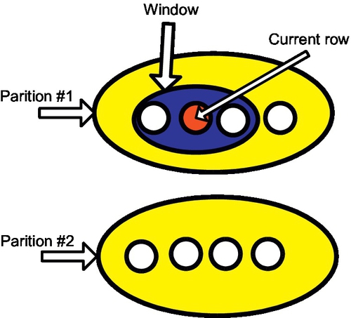
(1) EXCLUDE CURRENT ROW removes the current row from the window.
(2) EXCLUDE GROUP removes the current row and any peers of the current row.
(3) EXCLUDE TIES removed any rows other than the current row that are peers of the current row.
(4) EXCLUDE NO OTHERS makes sure that no additional rows are removed.
31.2.7 Windowed Aggregate Functions
The regular aggregate functions can take a window clause.
< aggregate function >
OVER ([PARTITION BY < column list >]
 [ORDER BY < sort column list >]
[< window frame >])
< aggregate function >::=
 MIN([DISTINCT | ALL] < value exp >) | MAX([DISTINCT | ALL] < value exp >)
| SUM([DISTINCT | ALL] < value exp >) | AVG([DISTINCT | ALL] < value exp >)
| COUNT([DISTINCT | ALL] [< value exp > | *])
There are no great surprises here. The window that is constructed acts as if it were a group to which the aggregate function is applied.
31.2.8 Ordinal Functions
The ordinal functions use the window clause but must have an ORDER BY subclause to make sense. They have no parameters. They create an ordering of the row within each partition or window frame relative to the rest of the rows in that partition. The ordering is not for the whole table.
31.2.8.1 Row Numbering
ROW_NUMBER() uniquely identifies rows with a sequential number based on the position of the row within the window defined by an ordering clause (if one is specified), starting with 1 for the first row and continuing sequentially to the last row in the window. If an ordering clause, ORDER BY, is not specified in the window, the row numbers are assigned to the rows in arbitrary order.
31.2.8.2 RANK() and DENSE_RANK()
RANK() assigns a sequential rank of a row within a window. The RANK() of a row is defined as one plus the number of rows that strictly precede the row. Rows that are not distinct within the ordering of the window are assigned equal ranks. If two or more rows are not distinct with respect to the ordering, then there will be one or more gaps in the sequential rank numbering. That is, the results of RANK() may have gaps in the numbers resulting from duplicate values.
DENSE_RANK() also assigns a sequential rank to a row in a window. However, a row’s DENSE_RANK() is one plus the number of rows preceding it that are distinct with respect to the ordering. Therefore, there will be no gaps in the sequential rank numbering, with ties being assigned the same rank.
31.2.8.3 PERCENT_RANK() and CUME_DIST
These were added in the SQL:2003 Standard and are defined in terms of earlier constructs. Let < approximate numeric type>1 be an approximate numeric type with implementation defined precision. PERCENT_RANK() OVER < window specification > is equivalent to:
CASE
WHEN COUNT(*)
OVER (< window specification >
 RANGE BETWEEN UNBOUNDED PRECEDING
AND UNBOUNDED FOLLOWING) = 1
THEN CAST (0 AS < approximate numeric type >)
ELSE (CAST (RANK ()
 OVER (< window specification >) AS < approximate numeric type>1) - 1)
/ (COUNT (*)
OVER (< window specification>1
 RANGE BETWEEN UNBOUNDED PRECEDING
AND UNBOUNDED FOLLOWING) - 1)
END
Likewise, the cumulative distribution is defined with an < approximate numeric type > with implementation defined precision. CUME_DIST() OVER < window specification > is equivalent to:
(CAST (COUNT (*)
OVER (< window specification >
RANGE UNBOUNDED PRECEDING) AS < approximate numeric type >)
/ COUNT(*)
OVER (< window specification>1
RANGE BETWEEN UNBOUNDED PRECEDING
AND UNBOUNDED FOLLOWING))
You can also go back and define the other windowed in terms of each other, but it is only a curiosity and has no practical value.
RANK() OVER < window specification > is equivalent to:
(COUNT (*) OVER (< window specification > RANGE UNBOUNDED PRECEDING)
-COUNT (*) OVER (< window specification>RANGE CURRENT ROW) + 1)
DENSE_RANK() OVER (< window specification >) is equivalent to:
COUNT (DISTINCT ROW (< value exp 1 >, . . .,<value exp n >))
OVER (< window specification > RANGE UNBOUNDED PRECEDING)
Where < value exp i > is a sort key in the table.
ROW_NUMBER() OVER WNS is equivalent to:
COUNT (*)
OVER (< window specification > ROWS UNBOUNDED PRECEDING)
31.2.8.4 Some Examples
The < aggregation grouping > defines a set of rows upon which the aggregate function operates for each row in the partition. Thus, in our example, for each month, you specify the set including it and the two preceding rows.
SELECT SH.region_nbr, SH.sales_month, SH.sales_amt,
AVG(SH.sales_amt)
OVER (PARTITION BY SH.region_nbr
ORDER BY SH.sales_month ASC
ROWS 2 PRECEDING)
AS moving_average,
SUM(SH.sales_amt)
OVER (PARTITION BY SH.region_nbr
ORDER BY SH.sales_month ASC
ROWS BETWEEN UNBOUNDED PRECEDING AND CURRENT ROW)
AS moving_total
FROM Sales_History AS SH;
Here, “AVG(SH.sales_amt) OVER (PARTITION BY…)” is the first OLAP function. The construct inside the OVER() clause defines the window of data to which the aggregate function, AVG() in this example, is applied.
The window clause defines a partitioned set of rows to which the aggregate function is applied. The window clause says to take Sales_History table and then apply the following operations to it.
1. Partition Sales_History by region
2. Order the data by month within each region.
3. Group each row with the two preceding rows in the same region.
4. Compute the windowed average on each grouping.
The database engine is not required to perform the steps in the order described here but has to produce the same result set as if they had been carried out.
The second windowed function is a cumulative total to date for each region. It is a very common query pattern or SQL idiom.
There are two main types of aggregation groups: physical and logical. In physical grouping, you count a specified number of rows that are before or after the current row. The Sales_History example used physical grouping. In logical grouping, you include all the data in a certain interval, defined in terms of a quantity that can be added to, or subtracted from, the current sort key. For instance, you create the same group whether you define it as the current month’s row plus:
(1) The two preceding rows as defined by the ORDER clause
(2) Any row containing a month no less than 2 months earlier.
Physical grouping works well for contiguous data and programmers who think in terms of sequential files. Physical grouping works for a larger variety of data types than logical grouping, because it does not require operations on values.
Logical grouping works better for data that has gaps or irregularities in the ordering and for programmers who think in SQL predicates. Logical grouping works only if you can do arithmetic on the values (such as numeric quantities and dates).
You will find another query pattern used with these functions. The function invocations need to get names to be referenced, so they are put into a derived table which is encased in a containing query
SELECT X.*
FROM (SELECT < window function 1 > AS W1,
< window function 2 > AS W2,
..
< window function n > AS Wn
FROM ..
 [WHERE ..]
) AS X
[WHERE..]
[GROUP BY ..];
Using the SELECT * in the containing query is a handy way to save repeating a select clause list over and over.
One point will confuse older SQL programmers. These OLAP extensions are scalar functions, not aggregates. You cannot nest aggregates in Standard SQL because it would make no sense. Consider this example:
SELECT customer_id, SUM(SUM(purchase_amt)) --error
FROM Sales
GROUP BY dept_nbr, customer_id;
But you may or may not be able to nest a windowed function in a regular aggregate. This will vary from SQL to SQL. If you get an error message, then use a CTE to get the windowed result set or look to grouping sets.
31.2.9 Vendor Extensions
You will find that vendors have added their own proprietary windowed functions to their products. While there is no good way to predict what they will do, there are two sets of common extensions. As a programming exercise, I suggest you try to write them in Standard SQL windowed functions so you can translate dialect SQL if you need to do so.
31.2.9.1 LEAD and LAG Functions
LEAD and LAG functions are nonstandard shorthands that you will find in Oracle and other SQL products. Rather than compute an aggregate value, they jump ahead or behind the current row and use that value in an expression. They take three arguments and an OVER() clause. The general syntax is shown below:
[LEAD | LAG] (< expr >, < offset >, < default >) OVER (< window specification >)
< expr > is the expression to compute from the leading or lagging row.
< offset > is the position of the leading or lagging row relative to the current row; it has to be a positive integer which defaults to one.
< default > is the value to return if the < offset > points to a row outside the partition range. Here is a simple example:
SELECT dept_nbr, emp_id, sal_amt,
LEAD(sal, 1, 0)
OVER (PARTITION BY dept_nbr
ORDER BY sal DESC NULLS LAST)AS lead_sal_amt,
LAG (sal, 1, 0)
OVER (PARTITION BY dept_nbr
ORDER BY sal DESC NULLS LAST) AS lag_sal_amt
FROM Personnel;
| Dept_nbr | Emp_id | Sal_amt | Lead_sal_amt | Lag_sal_amt |
| 10 | 7839 | $5000.00 | $2450.00 | $0.00 |
| 10 | 7934 | $1300.00 | $0.00 | $2450.00 |
| 10 | 7782 | $2450.00 | $1300.00 | $5000.00 |
| 20 | 7369 | $800.00 | $0.00 | $1100.00 |
| 20 | 7876 | $1100.00 | $800.00 | $2975.00 |
| 20 | 7566 | $2975.00 | $1100.00 | $3000.00 |
| 20 | 7902 | $3000.00 | $2975.00 | $3000.00 |
| 20 | 7788 | $3000.00 | $3000.00 | $0.00 |
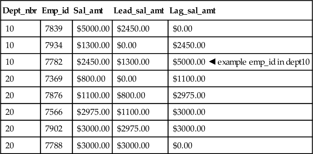
Look at employee 7782, whose current salary is $2450.00. Looking at the salaries, we see that the first salary greater than his is $5000.00 and the first salary less than his is $1300.00. Look at employee 7934 whose current salary of $1300.00 puts him at the bottom of the company pay scale; his lead_salary_amt is defaulted to zero.
31.2.9.2 FIRST and LAST Functions
FIRST and LAST functions are nonstandard shorthands that you will find in SQL products in various forms. Rather than compute an aggregate value, they sort a partition on one set of columns, then return an expression from the first or last row of that sort. The expression usually has nothing to do with the sorting columns. This is a bit like the joke about the British Sargent-Major ordering the troops to line up alphabetically by height. The general syntax is:
[FIRST | LAST](< expr >) OVER (< window specification >)
Using the imaginary Personnel table again:
SELECT emp_id, dept_nbr, hire_date,
FIRST(hire_date)
 OVER (PARTITION BY dept_nbr
ORDER BY emp_id)
AS first_hire_by_dept
FROM Personnel;
The results get the hire date for the employee who has the lowest employee id in each department.
| Emp_id | Dept_nbr | Hire_date | First_hire_by_dept |
| 7369 | 20 | ‘2011-01-01’ | ‘2011-01-01’ |
| 7566 | 20 | ‘2011-01-02’ | ‘2011-01-01’ |
| 7902 | 20 | ‘2011-01-02’ | ‘2011-01-01’ |
| 7788 | 20 | ‘2011-01-04’ | ‘2011-01-01’ |
| 7876 | 20 | ‘2011-01-07’ | ‘2011-01-01’ |
| 7499 | 30 | ‘2011-01-27’ | ‘2011-01-27’ |
| 7521 | 30 | ‘2011-01-09’ | ‘2011-01-27’ |
| 7844 | 30 | ‘2011-01-17’ | ‘2011-01-27’ |
| 7654 | 30 | ‘2011-01-18’ | ‘2011-01-27’ |
| 7900 | 30 | ‘2011-01-20’ | ‘2011-01-27’ |
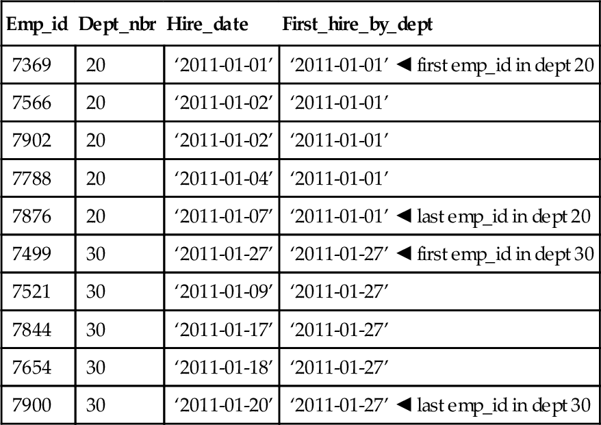
If we had used LAST() instead, the two chosen rows would have been:
(7876, 20, ‘2011-01-07’, ‘2011-01-01’)
(7900, 30, ‘2011-01-20’, ‘2011-01-27’)
The Oracle extensions FIRST_VALUE and LAST_VALUE are even stranger. They allow other ordinal and aggregate functions to be applied to the retrieved values. If you want to use them, I suggest that you look product-specific references and examples.
You can do these with Standard SQL and a little work. The skeleton
WITH FirstLastQuery
AS
(SELECT emp_id, dept_nbr,
ROW_NUMBER()
 OVER (PARTITION BY dept_nbr
ORDER BY emp_id ASC) AS asc_order,
ROW_NUMBER()
 OVER (PARTITION BY dept_nbr
ORDER BY emp_id DESC) AS desc_order
 FROM Personnel)
SELECT A.emp_id, A.dept_nbr,
OA.hire_date AS first_value,
OD.hire_date AS last_value
FROM FirstLastQuery AS A,
FirstLastQuery AS OA,
FirstLastQuery AS OD
WHERE OD.desc_order = 1
 AND OA.asc_order = 1;
31.2.9.3 NTILE Function
NTILE() splits a set into equal groups. It exists in SQL Server and Oracle, but it is not part of the SQL-99 Standards. Oracle adds the ability to sort NULLs either FIRST or LAST, but again this is a vendor extension.
NTILE(3) OVER (ORDER BY x)
The SQL engine attempts to get the groups the same size, but this is not always possible. The goal is then to have them differ by just one row. NTILE(n) where (n) is greater than the number of rows in the query, it is effectively a ROW_NUMBER(), with groups of size one.
Obviously, if you use NTILE(100), you will get percentiles, but you need at least 100 rows in the result set.
Jeff Moss has been using it for quite some time to work out outliers for statistical analysis of data. An outlier is a value that is outside the range of the other data values. He uses NTILE (200) and drops the first and 200th bucket to rule out the 0.5% on either end of the normal distribution.
If you do not have an NTILE(n) function in your SQL, you can write it with other SQL functions. The SQL Server implementation NTILE(n) function uses a temporary worktable that can be expensive when the COUNT(*) is not a multiple of (n).
The NTILE(n) puts larger groups before smaller groups in the order specified by the OVER clause. In fact, Marco Russo tested a millions row table and the following code used 37 times less I/O than the built-in function in SQL Server 2005.
Most of the time, you really do not care about the order of the groups and their sizes; in the real world they will usually vary by one or two rows. You can take the row number, divide it by the bucket size and find the nearest number plus one.
CEILING (ROW_NUMBER()
OVER (ORDER BY x)
/((SELECT COUNT(*) + 1.0
FROM Foobar)/:n))
AS ntile_bucket_nbr
This expression is like this non-OLAP expression:
SELECT S1.seq,
CEILING(((SELECT CAST(COUNT(*)+1 AS FLOAT)
FROM Sequence AS S2
WHERE S2.seq < S1.seq)/:n))
AS ntile_bucket_nbr
FROM Sequence AS S1;
Do not use this last piece code for a table of over a few hundred rows. It will run much too long on most products.
31.2.10 A Bit of History
IBM and Oracle jointly proposed these extensions in early 1999 and thanks to ANSI’s uncommonly rapid (and praiseworthy) actions, they are part of the SQL-99 Standard. IBM implemented portions of the specifications in DB2 UDB 6.2, which was commercially available in some forms as early as mid-1999. Oracle 8i version 2 and DB2 UDB 7.1, both released in late 1999, contain beefed-up implementations.
Other vendors contributed, including database tool vendors Brio, MicroStrategy, and Cognos and database vendor Informix, among others. A team lead by Dr. Hamid Pirahesh of IBM’s Almaden Research Laboratory played a particularly important role. After his team had researched the subject for about a year and come up with an approach to extending SQL in this area, he called Oracle. The companies then learned that each had independently done some significant work. With Andy Witkowski playing a pivotal role at Oracle, the two companies hammered out a joint standards proposal in about 2 months. Red Brick was actually the first product to implement this functionality before the standard, but in a less complete form. You can find details in the ANSI document “Introduction to OLAP Functions” by Fred Zemke, Krishna Kulkarni, Andy Witkowski, and Bob Lyle.