
CHAPTER 10
A Platform for Machine Learning
In the previous chapter, we talked about the Machine Learning model lifecycle. We saw how model development is a piece of the bigger puzzle that includes problem definition, data collection, cleansing, preparation, hyper‐parameter tuning, and deployment. A good data science or Machine Learning platform should provide tools that can drive automation in these different phases so that the data scientist can drive the end‐to‐end cycle without engagement with software development. This is like the DevOps for Machine Learning. Once the models are released in production, they should be consumed by software applications without special integration.
In this chapter, we will look at some tools and technologies that are being extensively adopted for building ML platforms. We will discuss the common concerns that a data scientist has to deal with while deploying an AI solution. We will see some of the best‐in‐class tools that address each of the concerns. We will also see how these individual products can be tied together to form a bigger data science platform hosted on Kubernetes.
Machine Learning Platform Concerns
We saw in the last chapter how the actual algorithm selection and model development is a key activity in solving an Artificial Intelligence problem. However, it is usually not the most time‐consuming. We have powerful libraries and platforms that simplify this activity and help us build and train models with a few lines of code. Some modern data science platforms actually let you select the right model and train without writing a single line of code. Model development and training with data is done purely through configuration. We see an example in this chapter of such a platform.
Data scientists typically spend more time addressing general concerns around collecting data, cleansing it, preparing it for model consumption, and distributing the training for the model and hyper‐parameters. Deploying the model to production is another major activity and mostly involves lots of manual interaction and translation work between the data scientists and software developers. Data scientists state that 50% to 80% of their overall solution development time is in activities not directly related to building or training a model—activities like data preparation, cleaning, and deployment. In fact, model development today is pretty well automated with libraries in languages like Python and R. However, the rest of the data science process still remains predominantly manual.
Major efforts are underway by top analytics‐consuming companies like Amazon, Google, and Microsoft in developing Machine Learning or data science platforms that can automate these different activities during the model development lifecycle. Examples of these platforms include Amazon SageMaker, Google AutoML, and Microsoft Azure Studio. These are usually tied to the respective Cloud offering of that particular provider. As long as you are okay with storing all your Big Data in the respective provider's Cloud (and paying for this), you can use their data science platform to ease up on the model development process. Depending on your specific requirements, you may find these Cloud offerings limited or may not want to store your data in a public Cloud. In that case, you can build an on‐premise data science platform of your own specific to your requirements.
We talk about the pros and cons of each approach. Either way, if your company is building and consuming a great deal of analytics, it is highly recommended that you invest in a Machine Learning platform that can ease up the software activities that are done by your data scientists.
In software development, an agile framework strives to add features to the product iteratively by releasing new code faster in short development cycles. This speed is achieved using automation tools like CI/CD, which take care of concerns like code compilation, running unit tests, and integrating the dependencies. In a similar manner, a data science platform will help you collect, access, and analyze data quickly and find patterns that could be deployed in the field for monetization. There are specific data science concerns that you want the platform to take care of, so your data scientists don't waste too much time doing this manually. Let's look at some of these concerns, outlined in Figure 10.1.

Figure 10.1: Typical data science concerns and tools that address them
Figure 10.1 shows some of the major concerns that a good data science or Machine Learning platform should address. I have been using these terms interchangeably because you will find both names used in industry. It is essentially a platform that helps data scientists address the concerns we see in Figure 10.1. Let's now look at these concerns and see how some of the leading tools address them.
Data Acquisition
Getting the right data to train your model is essential to making sure you are building a model that will work in the field. In most online tutorials or books on ML, you will see data already packaged as CSV files to be fed to the model. However, generating this neatly packaged CSV involves major effort and it will help the data scientist if the platform can take care of some of it. This involves connecting to the production data sources, querying the right data, and converting it into the desired format.
Traditional data sources used relational databases for storing large volumes of data. Structured Query Language (SQL) was the tool of choice to pull data from these databases. Relational databases store data in tabular format with tables that are linked to specific fields that are called the primary or foreign keys. Understanding the relationship between the data tables helps us build SQL queries that can pull the right data. Then we can store the results of the query in a manageable format like a CSV file.
Modern software systems often use Big Data technologies like Hadoop and Cassandra to store data. These systems form a cluster with many nodes, where the data is replicated across nodes to ensure fail‐over and high availability. These systems usually have a query language similar to SQL to collect the data. Again, knowing the structure of data is important to write the right query to pull data.
Finally, an emerging trend is to have data in motion. Data events occurring continuously are pushed to a message queue and interested consumers can subscribe and get the data. Kafka is becoming a very popular message broker for high‐frequency data.
A platform should be able to automatically connect to data sources and pull data. You do not need to worry about pulling data and building a CSV manually every time. A data science platform should have connectors to SQL, Big Data, and Kafka data sources so that data can be pulled as needed. This data collected from diverse data sources should be combined and given to your model for training. This should happen in the background, without manual intervention by data scientists.
One approach that is getting very popular is to use Kafka as the single source of input for all your data, from multiple sources. Kafka is a messaging system that's specifically designed for ingesting and processing data at a very high rate—in the order of thousands of messages per second. Kafka was developed by LinkedIn and then open sourced through the Apache foundation. Kafka helps us build data‐processing pipelines where we publish data packaged as messages to specific topics. Client applications subscribe to these topics and get notifications whenever new messages are added. This way, you decouple the publisher and subscriber of the data through the messaging system. This loose coupling helps build powerful enterprise applications. Figure 10.2 shows this process in action.

Figure 10.2: This Kafka‐based system for data ingestion includes a Hadoop connector for long‐term data storage
Figure 10.2 shows a Kafka broker with a topic where the data sources publish data wrapped as messages. A standardized format like JavaScript Object Notation (JSON) can be used to package your data and push this as a message. Typically, we create a topic of each data source so you can handle those messages differently. Kafka implements the publish‐subscribe mechanism—one or more client or consumer applications can subscribe to a topic of messages, and as new messages come onto the topic, the clients that are subscribed are notified. For each new message the client can write some handling logic to describe what needs to be done with the data that comes in with the message. As new data comes in, we could do analysis on the data, such as calculate summaries, trends, and find outliers. These analytics gets triggered as new data comes in as messages and Kafka notifies the subscribers of specific topics about the new data. As you notice, we can easily add more clients to the same topic or data source, so that the same data can be shared between multiple clients. This makes this architecture highly loosely‐coupled. Many modern software products follow this loosely‐coupled architecture.
We also see in Figure 10.2 that there is a special client or consumer that pushes data in the Hadoop cluster. Here the messages coming in are sent to a Hadoop cluster to store data long term. Hadoop is the most popular open source data processing framework for handling batch jobs. It follows a master‐slave architecture.
In Figure 10.2, we see a single master with six slave nodes. The master distributes data and processing logic across the slave nodes. In our example, along with the real‐time or streaming clients, we also send our data to a Hadoop cluster where it gets stored in the Hadoop distributed filesystem. Now we can use this stored data for running batch jobs. For example, every hour, we could run a batch job on the stored data to calculate averages and key performance indicators (KPIs). Hadoop also integrates very well with another open source framework for batch processing, called Apache Spark. Spark can also run batch jobs on a distributed Hadoop cluster, but these jobs run in memory and are very fast and efficient. Other Big Data systems like Cassandra have ways to store data in a cluster and apply ML models to this data and extract results.
In this example, we see two scenarios for Big Data processing. We see real‐time or streaming data processing using Kafka. We build subscribers for specific topics that consume the data and apply specific analytics on this data. We also see this data stored in a Hadoop cluster for long‐term storage and applying ML models on this data in a batch mode.
Irrespective of the original data source, all data is converted to a common format and can be easily consumed by our analytic models. This pattern of decoupling the source of data from the consumer greatly simplifies your data science workflow and makes it highly scalable. You can quickly add new data sources by having them add data to an existing queue in an agreed‐upon common format. Modern data science platforms typically support connectivity to these streaming and batch processing systems. You could have a platform like AWS SageMaker pull data from a Kafka topic and run your ML model or connect to a Hadoop data source (hosted on AWS) and read data to train your model.
Another trend that is emerging in the industry is having something called a gold dataset. This is a dataset that perfectly represents the kind of data the model will see in the field. Ideally it should have all the extreme cases, including any anomalies that need to be flagged. For example, say your model is looking at stock prices and making buy vs. sell decisions. If there are historical accounts of significant market rises or crashes, we will want to capture these cases and the corresponding buy or sell decisions (respectively) in our gold dataset. Any new model we develop should be able to correctly predict these patterns so that we know they function well. Typically, a gold dataset will consist of obvious cases that the model should predict for before being able to move to more complex patterns. We can also include validation against the gold dataset as a precondition for deployment into production, as part of our ML continuous integration process.
Data Cleansing
Data cleansing is all about getting rid of any noise in the data to make it ready to feed to the model. This could involve getting rid of duplicate records, imputing missing data, and changing the structure of data to fit a common format. Data cleansing may be done in Microsoft Excel by loading a CSV and applying simple search and filtering tools, although this is the most basic form and almost never done in true production environments. The volume of data in real‐world systems cannot be handled in tools like Excel. We typically cleanse data using specialized streaming or batch jobs that contain rules for handling missing or bad data.
As we saw in the previous section on data collection, we could have a unified Kafka broker that serves us data from several different data sources. Now we could subscribe to these topics and write our logic to cleanse the data and write back the cleansed data to a new queue. The cleansing may be done in a batch job on data stored in Hadoop using a batch job processing framework like Spark.
There are also some dedicated tools that do data cleansing. A popular such tool is called Tamr and it internally uses AI to match data. It works on the Unsupervised Learning principle, where it tries to identify clusters of similar data and applies common cleansing strategies on this data. Another tool that has similar capabilities is called Talend. It is more deterministic and does cleansing based on predefined rules. These tools also connect to data sources like Hadoop and Kafka and provide cleansed data to build the ML model.
Another common problem with large systems with many data sources is a lack of master data. You have the same information replicated at multiple places and there is no standard identification field to relate the data. Common data fields like customer names and addresses are often stored in different ways in different systems, which causes problems while searching. Hence, large enterprises employ a Master Data Management (MDM) strategy, where data from specific data sources is considered a reference and used to represent the single source of truth. All systems use this as standard and work around it. This MDM system can serve as an excellent input for training ML models and should be considered for integration with the data science platform. Talend and Informatica are very popular MDM systems that help combine diverse data sources and establish a single source of truth to be used by downstream applications.
Analytics User Interface
The user interface for analytics should be intuitive and provide easy access to run descriptive statistics on our data. It should provide access to data sources like SQL and Kafka either programmatically or through code. It should allow us to try different ML algorithms on our data and compare the results.
Web‐based user interfaces that can be opened in a browser have become the standard for building modern analytics models. Jupyter Notebooks is an open source solution that has been adopted by many data science platforms, including Google's Colaboratory (which you used earlier) and Amazon SageMaker. Jupyter provides a very intuitive programmatic interface for experimenting with data and running your code to get immediate results. Because Jupyter Notebooks is launched from Python, you can create an environment with all the necessary Python libraries and make them available from inside the Notebook. Now your Notebook can run a lot of these complex function calls without having to explicitly install these libraries. We saw an example of this in the previous chapter, when we ran custom code for running a model on a TPU in the Notebook provided by Google Colaboratory.
A couple of startups that have been working on a powerful configurable user interface for data science are H2O.ai and DataRobot. They provide very powerful user experiences that allow linking to data sources and model development without writing a line of code. These were still in the startup stage as of 2018, and we don't know how much they will grow by the time you are reading this book. Maybe one of them will become the de‐facto UI tool for building ML models!
Let's now take a quick look at how H2O.ai allows us to build models without writing a single line of code. The interface may change, but I want to focus your attention on the thought process of simplifying the data science process for engineers. H2O is a distributed Machine Learning framework. It tries to address a few of the data science concerns we talked about earlier. It includes an analytics UI called H2O Flow and a Machine Learning engine that has support for some of the top supervised and unsupervised algorithms. It also provides support to store data in a cluster and distribute ML jobs on the cluster.
H2O is open source and freely available. You can download and run it on your local machine or get a Docker image from H2O.ai. Its only dependency is Java—it is basically a Java application on its own. I won't go into detail about installation and setup. I will show an example of building a model with custom data. The data I download is the wine quality dataset that is publicly available as a CSV file. The model built in H2O with this data file is shown in the next section—notice the ease of use in the user interface.
Developing an ML Regression Model in H2O Without Writing a Single Line of Code
H2O is a modern data science platform developed by the company H2O.ai. H2O allows users to fit thousands of potential models as part of discovering patterns in data. The H2O software runs can be called from the statistical package R, Python, and other environments. H2O also has an extremely intuitive web UI called H2O Flow that allows you to import data, build a model, and train it inside a web browser without writing a single line of code. All this is done using the web‐based UI and its configuration. We will see an example next. To install H2O, follow the steps at this web link: http://h2o‐release.s3.amazonaws.com/h2o/rel‐xu/1/index.html.
You can install H2O as a standalone Java application or as a Docker container. After installing H2O as a standalone or Docker container, launch the web UI. You can explore different menus and help options in the web UI. For uploading your CSV file, select the Upload File option from the Data menu. H2O also supports connections to SQL databases and Hadoop Distributed File System (HDFS). The H2O web UI is shown in Figure 10.3.
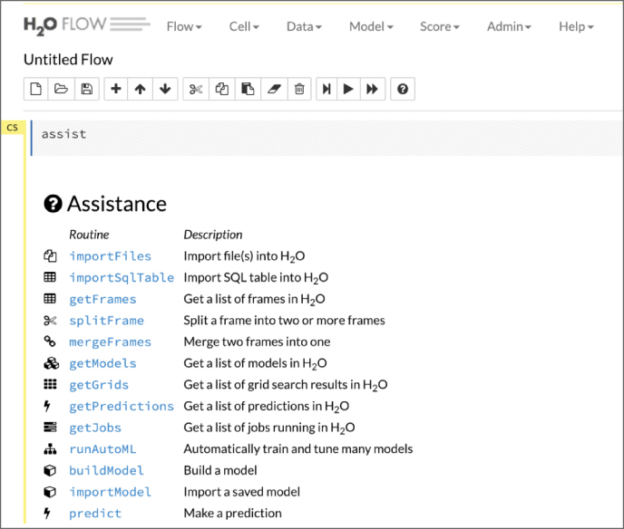
Figure 10.3: H2O web user interface (UI)—Flow
Now let's use the wine quality CSV file and upload it (see Figure 10.4). Once the CSV file is uploaded, the tool will automatically parse the columns and extract the data. It will show you what fields or columns are available and what the datatype is. You can modify the datatype—for example, you can change numeric to categorical. If you have wine quality as an integer value between 0 and 10, it's better to convert it to categorical. Then by the click of a button, you can parse this CSV file and store the data in a compressed binary data structure called a data frame. The beauty of the data frame is that it is a distributed data structure, so if you have a five‐node cluster, for example, you can store data distributed across this cluster. You don't have to worry about the distributed data storage concern—the tool takes care of that.

Figure 10.4: Uploading and parsing a CSV file—no code needed
H2O also has an easy interface to split the data into training and validation data frames. That way, when you build the model, you can specify what data frame to use for training and which one for validation. You can specify the percentages you want to use to distribute your data into training and validation—typically this is an 80‐20 or 75‐25 split. See Figure 10.5.

Figure 10.5: Checking the parsed data frame and splitting it into training and testing sets
Once you have the data frames defined, go to the Model menu and select the algorithm you want to use. H2O (as of 2018) provides modeling options for several popular algorithms, including generalized linear models, random forests, etc. It also supports Deep Learning but for structured data. You select a model type, training and validation frames, and the output feature you want to predict. Based on selected model, the appropriate hyper‐parameters are populated. Each hyper‐parameter has a default value and you can modify that as needed. The selection of the correct hyper‐parameters is a major concern that data scientists have to deal with. Usually, with experience, you develop some rules of thumb for selecting the right hyper‐parameters based on your problem domain and the type of data being handled. See Figure 10.6.

Figure 10.6: Selecting the model and defining hyper‐parameters for it
Then you can submit the job for training the model, which builds the particular model. The tool also shows the accuracy parameters on the training and validation datasets you selected during configuration. In Figure 10.6, we selected a generalized linear model (GLM) and it shows us how much each variable (X) affects the dependent variable (Y)—in this case the quality of wine. You can see that this model was built, configured (hyper‐parameters), and trained without writing any code purely through the configuration UI. That's the power H2O brings. Of course, coding will give you a lot more flexibility, but H2O is a great way to get familiar with the different aspects of ML. See Figure 10.7.
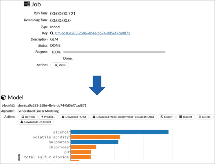
Figure 10.7: Running the training job. Evaluating the trained model. Still no code written!
The model created can then be exported as a binary file. You can write Java code to call this binary file to run the model. This code can also be packaged as a web application and deployed as a microservice. This method of model deployment is gaining immense popularity in the industry.
That's the end of our small sidetrack to show an H2O example. Let's get back to discussing other major concerns the data scientist usually has to deal with.
Model Development
We saw how a platform like H2O takes care of the model building concerns by using an intuitive web‐based UI for model development. You can host H2O or Jupyter Notebooks on a cluster of extremely powerful servers with many CPUs, memory, and storage. Then you can allow data scientists from your company, or maybe from across the world, to access the cluster and build models. This will save on the huge investment in giving individual data scientists powerful machines and licenses (like MATLAB) for model development. This is the most popular pattern today in companies that are big on analytics. It enables them to have a centralized common model development user interface that can be accessed by thin clients like web browsers.
If you are building models programmatically in Python, the library of choice is Scikit‐Learn for shallow Machine Learning models. For Deep Learning, it's better to have a framework that allows you to build computation graphs representing the neural networks. Popular frameworks are TensorFlow by Google and PyTorch by Facebook. Both are free and open source, and can help build different feed‐forward and recurrent network architectures to help you solve the problem in your domain. We typically call these frameworks because they don't just get plugged into an existing runtime, but come with a full runtime of their own. The frameworks allow developers to connect to their runtime and run training jobs using their language of choice, like Python, Java, or C++. When you build a TensorFlow model, it runs in a separate session on its own cluster, which may be composed of CPUs or GPUs.
Typically, many popular tools are available for model development with good documentation. This is the one concern that usually gets the most attention.
Training at Scale
For small demo projects and proofs of concept, you will mostly have limited data in a common format like CSV and build a quick model to see how well it fits on this data. However, the bigger the training data, the more generalized your model will be. In the real world, the data volumes will be very high and the data will often be distributed on a cluster using a framework like Hadoop. When you have large volume of data you most likely need a way to distribute your model training on a cluster to take advantage of the distributed nature of data. We saw the H2O training example earlier and it would automatically distribute your training job on the cluster. H2O captures this pattern very well but you need to be inside the H2O ecosystem to utilize it. There are other tools available that focus on addressing this concern of training at scale.
The Spark framework has an MLLib module that allows us to build distributed training pipelines. Spark has interfaces in Python, C++, and Java so you can write your logic in any language and get it running on the Spark framework. The idea behind Big Data frameworks like Spark and Hadoop is that you push the computing where the data is. For huge volumes of data distributed in a cluster, it's highly time‐consuming to collect data centrally for processing. Hence the pattern here is to package your code and deploy on individual machines where the data exists and then collect the results. All this processing of data at the machines where data resides happens in background and end user has to write code just once. The Spark MLLib module usually is good for Machine Learning algorithms.
TensorFlow for Deep Learning also provides support for distributed model training. After creating a computational graph, you run this in a session, which may be run in a distributed environment. The session may also be run in a highly parallelized environment like a GPU. As we saw in the previous chapter, a GPU has thousands of parallel processing cores, each dedicated to performing linear algebra operations. Collectively, these cores help in running Deep Learning calculations in parallel and train models faster than on a CPU.
Google is also developing a TensorFlow distributed training module for Kubernetes, called TFJob. We will talk about this more in the last part of this chapter.
Hyper‐Parameter Tuning
Typically, data scientists spend most of their time trying different hyper‐parameters like the number of layers, neurons in a layer, learning rate, type of algorithm, etc. We talked about hyper‐parameter tuning in the previous chapter. Usually, data scientists develop best practices for selecting hyper‐parameters for a specific problem or dataset at hand. Tools like H2O capture some of these best practices and give recommendations. You can start with these recommendations and then search for better fitting hyper‐parameters.
A new methodology, called AutoML, is evolving that automatically finds the best hyper‐parameters by searching through many combinations in parallel. AutoML is still an evolving area. As it matures, this is surely going to save data scientists a lot of time.
H2O has an AutoML module in the Model menu that runs different types of models with different hyper‐parameters in parallel. It shows a leaderboard with winning models. Google has a Cloud AutoML offering where you can upload your data like images and text and the system selects the right Deep Learning architecture with the right hyper‐parameters. Let's quickly look at the AutoML module in H2O, discussed in the following section.
There is a new tool emerging on top of Keras called AutoKeras. It provides an AutoML interface for a Keras model. So now we can tune the hyper‐parameters in a Deep Learning model and select the ones that give us the most accurate numbers.
H2O Example Using AutoML
We will continue with the earlier example of using the H2O web UI for regression analysis on the wine quality dataset. We will select the AutoML technique that H2O offers and see if it helps us. We first select the AutoML option and then select the training and validation data frames. See Figure 10.8.
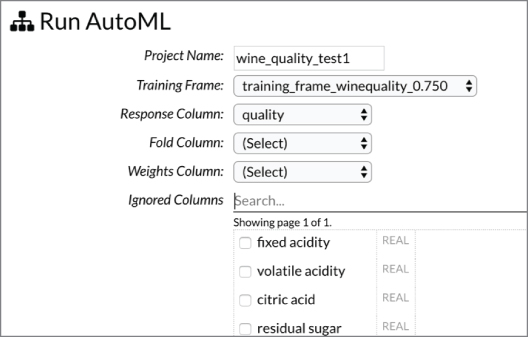
Figure 10.8: Selecting Run AutoML from the menu bar
Now we run the AutoML job. It will take a few minutes to run and show the progress on a progress bar. Once a significant number of models are run in parallel, we will get a leaderboard that compares the results. See Figure 10.9. Here we have regression, hence the mean_residual_deviance is used as the metric to score the model on the leaderboard. Any of the models on the leaderboard may be downloaded as binary and deployed.

Figure 10.9: Running the AutoML job. Note the leaderboard of all different models compared for your datasets.
Automated Deployment
During model development, there are two main areas that can be automated—training the model and inference of new data. Training involves tuning the weights using the training dataset so the model can make accurate predictions. Inferencing is feeding new data to the model and making predictions. We developed a web application in the last chapter that feeds data to a trained model, makes the inferences, and shows the results in an application. This will work for a small application with basic models. However, for large applications, we need loose coupling between the software code and the model.
The most popular method of creating this loose coupling is using the microservices architecture pattern. The model gets packaged as a container and deployed as a microservice that gets called with lightweight HTTP requests. This can be done using a custom application like we did in Chapter 7 or using an automated deployment framework. Machine Learning model deployment frameworks are still evolving. Amazon SageMaker has a deployment engine that's very specific to AWS. There are a few openly available model serving frameworks that you can plug into your data science platform. Let's look at some of these.
A popular open source deployment and inference engine is provided by Google called TensorFlow‐Serving (TF‐Serving). Despite the name, TF‐Serving is pretty flexible and can also deploy normal ML models developed in Scikit‐Learn. The only catch is that the model should be available in Google's open prototype buffer format. The model should be saved as an extension PB file and can then be deployed as a microservice in TF‐Serving. You can manage different versions of a model and TF‐Serving will load these and allow you to invoke them with separate URLs.
Another popular inference engine that is evolving is NVIDIA's Tensor‐RT. This is becoming very popular for running models very fast at the edge. It is also gaining traction for server and Cloud model deployments. Tensor‐RT is not related to TensorFlow—it allows models developing in different Deep Learning frameworks to be deployed and inferred upon. The models must be converted into Tensor‐RT binary format before deployment. Compared to running inference using native TensorFlow, we usually get around 10x improvement with Tensor‐RT. This is because Tensor‐RT re‐creates the Deep Learning models by applying several optimizations and with more compact architectures. Tensor‐RT is available as a Docker‐based containerized microservice that you can deploy in your environment.
TF‐Serving is available as a Docker image in DockerHub. You can use this image to build containers that serve as microservices serving packaged models. Models are packaged into the prototype buffer format with a specific folder structure. Let's see how to do deployments. We will use a very simple example of TensorFlow code to build a basic computational graph. We will not use Keras because we don't have a deep network with many layers. We will just do basic operations to illustrate the concept.
Listing 10.1 shows the code for a simple computation graph that takes two input variables (x2, x2) and calculates an output (y).
If you run this file, it will create a folder called /tmp/test_model/1 and save the model we just created inside the folder. This was a deterministic model that will always give the same output. We could capture complex patterns and build this model.
Now we will create a container with the TensorFlow‐Serving image and try to invoke our model through a REST API. The TensorFlow‐Serving image is available in the open DockerHub repository and can be downloaded. We will run the Docker container from the image and pass the folder where we developed the model as a parameter. We will also map a network port from the container to our machine so that you can access the microservice by calling the host machine. The TensorFlow‐Serving will wrap our model and make it available as a microservice. See Listing 10.2.
Notice that we passed the model folder and name. Also, we mapped port 8501 to our local port. The image name is tensorflow/serving. Now you can invoke this model directly using REST API calls, as shown here:
$ curl -d '{"instances": [{"x1":2.0,"x2":3.0},{"x1":0.5,"x2":0.2}]}' -XPOST http://localhost:8501/v1/models/test_model:predict{"predictions": [80.0, 9.0]}
We call the URL of the model exposed by TensorFlow‐Serving. We pass JSON data indicating the number of points to process—instances—and for each, the values of variables x1 and x2. That's it. We can pass more data packaged as the JSON and the image will be served as a container. The result is a JSON string with the values of predictions. The same can be done for Deep Learning models with libraries like Keras.
Deployment of DL Models in Keras
The previous section was a very basic example of a computational graph in TensorFlow that we deployed as a microservice—not very impressive. Now let's take a Deep Learning model and “serve” it and invoke it using a client application. We will use the Keras model created in Chapter 5 for classifying between Pepsi and Coca‐Cola logos. If you recall—we saved this model as an HDF5 file called my_logo_model.h5. We will save this file in a folder and run the code in Listing 10.3 to convert it into the prototype buffer format that TensorFlow‐Serving expects.
Typically to do this sort of conversion it's better to write a generic utility file rather than custom code each time. Let's write a utility that will take the H5 file, output the model name and version as parameters, and convert your H5 file into a versioned model that we will later serve.
You can choose any language to write this utility as long as it can handle command‐line parameters and call TensorFlow libraries. I will use Python for this. Listing 10.3 shows the code.
You can use this utility and it will generate your PB file. Digging into the code, you will see that it ensures that you have passed the right parameters for the H5 file and the model name and version. Also, it verifies that the same model and version do not exist. It's a good idea when you're writing any code to check for failure modes like this. It greatly improves the reliability of your code. You never know what the user will enter for these inputs.
Then the code loads the Keras saved model from the H5 file. Since Keras runs on top of TensorFlow, this model is also automatically loaded in a TensorFlow session object. All we have to do now is save this session object and we have our prototype buffer file. That's what we do and we have the model ready for serving. TensorFlow‐Serving takes the structure of <Model_Name>/<Version> for the folder structure. This allows you to manage the versions of your model better.
Now let's use this utility to convert the my_logo_model.h5 file from earlier. We put the file in the same folder where we run this Python script and then run the code shown in Listing 10.4.
We pass the model H5 file and output the model name and version as parameters. The result will be a new folder, called my_logo_model/1, which contains the PB file and a variables folder:
$ ls my_logo_model/1/saved_model.pbvariables
Now we will create a Docker container like we did earlier using the tensorflow/serving image. This container will host our model and expose an HTTP interface to call our model. We don't have to write any custom application code—all the piping for exposing the REST API is taken care by TensorFlow‐Serving:
$ docker run -it --rm -p 8501:8501 -v '/my_folder_path/my_logo_model:/models/logo_model' -e MODEL_NAME=logo_model tensorflow/servingAdding/updating models.Successfully reserved resources to load servable {name: logo_modelversion: 1}....Successfully loaded servable version {name: logo_model version: 1}
We now have our logo detection model loaded in TensorFlow‐Serving to serve as a microservice. In the earlier example, we used the CURL command to call our model microservice and pass parameters. In this example, we have to pass a whole 150×150 sized image to the model. For this, we use Python to load the image and call our service. Listing 10.5 builds a client that does exactly this.
Figure 10.10 shows the images we used for our test (test1.png and test2.png).

Figure 10.10: Images used to validate the model
OUTPUT:Prediction for test1.png = {'predictions': [[1.23764e-24]]}Prediction for test2.png = {'predictions': [[1.0]]}
We see that for the Coke image (test1.png), when we pass the image to our model, it gives a prediction close to 0 and for the Pepsi image (test2.png), it gives the value of 1. That's how we trained the model and we see good results. You can also use images downloaded on the Internet and see the results.
Keep in mind that the client code we ran does not have any direct TensorFlow dependency. We take the image, normalize it (dividing by 255), convert it to a list, and pass it to our REST endpoint. The result comes back as a JSON value that can be decoded to get our result as 0 or 1. This is a binary classification; hence, we just have 1 result with 0 or 1 outcomes. Practically, you will build more complex models that will do multi‐class predictions. These can also be hosted on TensorFlow‐Serving.
We have seen how a major concern for data scientists—deployment of models at scale—can be handled using TensorFlow‐Serving. As we saw earlier, since TensorFlow‐Serving runs as a Docker container, we can easily package it as a deployment in Kubernetes and scale the deployment to multiple pods. Kubernetes will handle the scaling and fail‐over to handle large client loads. You will have to create a volume for storing your model files. Kubernetes includes concepts like persistent volumes and persistent volume claims that can take care of this.
Let's return to another major concern for data scientists—logging and monitoring—and discuss how we can take care of them using this platform.
Logging and Monitoring
Finally, the two most common concerns among all types of software applications relate to logging and monitoring. You need to be able to continuously monitor your software application to catch and log errors, such as out‐of‐memory errors, runtime exceptions, permission errors, etc. You need to log these errors or items of interest so that the operations team can identify the health of your software or model. Your application or microservice that serves the model also needs to be monitored so that it is available for clients. If you use a platform like Kubernetes, it comes with log‐collection and monitoring tools that help address these concerns. The deployment platforms like TensorFlow‐Serving and Tensor‐RT have logging built in and can give you quick outputs.
Monitoring and logging concerns are typically passed on to a platform like Kubernetes. If we deploy our model training and inference microservices on Kubernetes, we would use a monitoring tool like Prometheus and a logging tool like Logstash. Both of these can also be deployed as microservices on the same Kubernetes cluster.
Putting the ML Platform Together
In the previous section, we saw how tools are available to address specific data science concerns. We also saw how Kubernetes can act as a single unified platform for addressing software application concerns. By extending Kubernetes, we can also address these data science concerns. Because a lot of the tools we saw earlier can be packaged as microservices, we could host specific microservices to enable Kubernetes to handle data science requirements. This extension is done by an open source project being developed at Google, called Kubeflow.
Kubeflow allows easy and uniform deployment of Machine Learning workflows on a Kubernetes cluster. The same ML deployment pipeline can be done on a local MiniKube, an on‐premise Kubernetes cluster, and a Cloud‐hosted environment.
Kubeflow takes industry‐leading solutions to address many data science concerns and deploys them together on Kubernetes. I will not talk about Kubeflow installation on a Kubernetes cluster, mainly because these instructions keep changing as the product is being stabilized. You can get the latest instructions at Kubeflow.org.
Once Kubeflow is installed in its namespace, you can list the deployments and services in that namespace to see what was installed. Kubeflow is a high‐level application that is installed on Kubernetes and it installs all specific microservices. Kubeflow by itself does not solve any data science concerns but works on integrating individual components.
At a bare minimum you should see JupyterHub (Analytics UI), TF‐Job (Model training), and TF‐Serving (Deployment) components. You can start with the Jupyter Notebooks to build the model and submit it to the TF‐Job to schedule a distributed training job. Once you have model trained you can deploy it using TF‐Serving as a microservice on the Kubernetes cluster. Clients can call HTTP API to invoke the model and run inference. TF‐Serving also supports Google's gRPC protocol, which is significantly faster than HTTP. gRPC packages data in binary format and takes advantage of HTTP/2 to handle unstructured data, like images.
As you see, Kubeflow is not a complete solution by itself; it's more like the glue that gives us a standard interface to integrate ML components on Kubernetes. Over time, more and more components will get added to Kubeflow and will be easily deployable on Kubernetes. If you are building your own platform for data scientists, Kubeflow on Kubernetes should definitely be on the top of your list.
Summary
In this chapter, we talked about the major common concerns affecting data scientists, like data cleansing, analytics UI, and distributed training. We looked at some industry standard tools—like TensorFlow‐Serving and Jupyter—for addressing specific concerns. Then we looked at an upcoming technology called Kubeflow, which provides a standard way to deploy ML workloads on Kubernetes. We also saw an example of deploying a simple TensorFlow analytic using TF‐Serving.
That's it folks, for now. We saw basic concepts of Machine Learning and Deep Learning. We learned how to handle structured and unstructured data. We developed DL models for analyzing text and image data using a popular library called Keras. We developed models to classify soda logo images and identify sentiment from text. We also saw some cool examples of making AI models create paintings and generate new images. In the second half of the book, we looked at packaging the models into microservices and managing their deployment. We looked at different data science concerns like data collection, cleansing, preparation, model building, hyper‐parameter tuning, distributed training, and deployment. Finally, we learned about Kubeflow, which is an upcoming technology to deploy ML workflows on Kubernetes.
A Final Word …
All the code from this book is available on this GitHub link: https://github.com/dattarajrao/keras2kubernetes.
Hopefully this book has given you a holistic picture of building AI models and deploying these at scale in production environments. Often times we see data scientists focus on the algorithm development and don't have enough tools in their repertoire to handle other concerns like data cleansing, distributed training, and deployment. As we saw, this technology is still being developed. There is huge opportunity in this space and new solutions coming up. Hopefully this book has triggered your interest in this space and you will be able to leverage the right tools when you face these problems. Do write to me with any feedback and comments about the book. Here's wishing you all the best on your real‐world Machine Learning journey!