
CHAPTER 2
Machine Learning
Chapter 1 provided an overview of some of the emerging trends in the industry around Big Data and Artificial Intelligence. We talked about software getting smarter with the application of Artificial Intelligence. In this chapter, we specifically focus on the most popular AI technique for infusing smarts into software—Machine Learning (ML). We see examples of using ML to capture patterns in data and capture these patterns in artifacts called models. We see the three types of ML techniques and discuss applications of each. Finally, in this chapter we review some code examples of building ML models from simple datasets. The code is highly commented, so you can start your own Colaboratory or Jupyter Notebook environment and run the code.
Finding Patterns in Data
As you saw in Chapter 1, AI is all about making computers develop human‐like intelligence. This intelligence can help computers do knowledge representation, learning, planning, perception, language understanding, and more. One of the key areas of AI is Machine Learning, which is all about finding patterns in the data. The human brain is excellent at finding patterns. However, it is not very good at handling lots and lots of data.
Let's look at an example in Listing 2.1. Can you correctly guess the next number in the series?
You should have no trouble looking at this data and finding the pattern. This is the powerful natural intelligence your brain has. You see that they are all even numbers in increments of 2. To capture this pattern in data, all the machine needs to do is build a rule that says add 2 to the previous number and that's the next number. Pretty simple, huh?
Wait a minute. Some of you may have noticed that the number 26 is missing in this sequence. Our brain is great at finding patterns but as we process more data we tend to miss things. If there is too much data, we usually get things wrong over time due to human error and fatigue. In this simple example, some of you may have actually noticed the missing 26 and probably attributed it to a printing mistake—but its omission was intentional!
Now look at the set of numbers in Listing 2.2. We are no longer dealing with integers but with real numbers with decimal points. This makes it more difficult.
Just by looking at this sequence, it's pretty difficult for our brains to find patterns. We can make some sense of the data increasing and decreasing but cannot do much with it. Now for a computer, this new data is almost the same as the previous list of integers. With a minimal increase in processing power, a computer can analyze this new data. However, it still needs a human‐like capability to find the pattern. In other words, it needs some level of Artificial Intelligence to find a pattern. This is where Machine Learning (ML) comes in the picture. So why is ML a big deal? If we train computers to find patterns in huge volumes of Big Data without getting tired and making human‐like mistakes, we can get lots of intelligent work done quickly and highly accurately.
Now let's plot the data from the previous example and see what we find. No coding or any fancy tools. We will only use Excel. We take these numbers and plot the points on a chart in Excel. Immediately we see a pattern emerging. The values increase and decrease periodically and form a wave. So, there is a prominent pattern in the data and we only see this with help of a visual aid—a chart (see Figure 2.1).

Figure 2.1: Charting these real numbers shows a pattern
Many business intelligence and reporting tools work on this basic principle—they process data, calculate important statistical summaries, and show results on intuitive visual aids (mostly charts) that help us understand the data and look for patterns. However, they still rely on humans to make the final decision by processing all this information. This approach is usually referred to as descriptive analytics.
Machine Learning goes beyond descriptive analytics, into the realm of predictive analytics. We find patterns in data and store these patterns in an artifact called a model. The model can now be used for making predictions on new data. The process of building a model is called training. Even before we start actually training, we need to collect data and identify the algorithm we will use for training.
In order to make accurate predictions on the new data, our model needs to learn all the patterns in the data. It needs to understand all the variations that the real data will encounter. Otherwise, it will have limited capability and will be less accurate. Also, the quality of data used to build the model is very important. Here ML follows the GIGO—Garbage In Garbage Out—rule. You need to feed the model with good data, or it will learn incorrect patterns.
Take the earlier example of integers. If we had fed the ML model with a sequence with the missing 26, it would think that it is a true pattern and start learning that. That would affect the accuracy of the model. There are more steps in the ML model lifecycle. We usually focus on the algorithm, but equally important (and sometimes more important) are the data collection, preparation, and model deployment and monitoring steps. The real world keeps changing, so a model deployed in production may not be relevant over time due to changes to the environment. A solid monitoring strategy and feedback cycle is very important when you deploy ML models in production. We will talk about this issue in the next chapter.
Let's focus on some of the popular algorithms and techniques in ML. Here I describe some common techniques in simple terms with examples and sample code. I also provide links for websites that provide these techniques in details.
The Awesome Machine Learning Community
Before we start—a word on the Machine Learning community. The ML community is truly amazing and provides a huge amount of data and information for free. They publish an amazing amount of content regarding algorithms and techniques and most of it is available for free. Many times it includes sample code. It's a really fun discipline to learn with lots of involvement across the globe. You can find many magazines, articles, and communities open to listening to your problem and helping with solutions.
Moreover, websites like Kaggle.com host ML competitions where they provide real‐world problems with sample datasets (see Figure 2.2). Anyone in the world can register and join these competitions and be in line to win thousands of dollars. They don't care which country you are from or what your academic background is—the only thing that matters is how well you can solve the data science problem. Truly making the world a much smaller place!

Figure 2.2: Kaggle hosts data science competitions and gives free datasets
(Source: kaggle.com)
For explaining the different algorithms, I use some publicly available datasets.
Again, thanks to the amazing ML community, we have many good datasets that can be used for learning ML methods. We will use datasets provided by the University of California, Irvine's Center for Machine Learning and Intelligent Systems (see Figure 2.3).

Figure 2.3: UCI Machine Learning repository
(Source: uci.edu)
Types of Machine Learning Techniques
Machine Learning is that one field of AI that touches and influences almost every other discipline. In fact, in the last five years there is hardly any area of the consumer and industrial Internet that has not been transformed by ML. All the AI examples we saw earlier—like tagging photos, recommender systems, playing games like chess, and self‐driving cars—use some form of learning methods. ML can be classified into three areas, discussed in the following sections.
Unsupervised Machine Learning
In this case, we do not have any data on the results that are expected from our analysis. This is a more classical approach to finding patterns and trying to determine what the data is “telling” us. We focus on finding generic patterns in the dataset and using these to gain insights. Unsupervised learning algorithms can be divided into three categories.
Clustering
Clustering is all about dividing the dataset into clusters or groups with similar characteristics. Based on the variation in data in different features/columns, we try to determine what data points are similar and put them in a cluster. For example, if we have a class of students with different heights, we could divide them into tall, medium, and short categories. Clustering techniques analyze the data statistically to find groups of similar points. Let's discuss some common clustering methods.
K‐Means is a popular method where you specify K number of clusters and the algorithm finds optimal clusters by assigning points to each cluster by distance from the centroid of each cluster. We will see a code example of clustering later in this chapter, when we analyze a dataset of houses using the K‐Means algorithm.
Another popular algorithm is called DBSCAN (Density‐Based Spatial Clustering of Applications with Noise). With it, we don't need to specify the number of clusters as in K‐Means. The algorithm finds regions in feature space where the density of points is high. Other popular clustering algorithms include Hierarchical Clustering and t‐SNE (t—Distributed Stochastic Neighbor Embedding). Each has a different way of finding clusters, but the basic idea is the same—they find data points that are statistically similar and group them as a cluster.
Dimensionality Reduction
Another popular unsupervised learning method is called dimensionality reduction. The idea here is to reduce the number of features/columns in your dataset. Too many features are difficult to handle and visualize. Also, you may end up focusing on features that are not of interest. For example, if we have 10 features describing a medical dataset—maybe 10 measurements of a sample of patients like blood pressure, cholesterol, sugar, etc.—it would probably be easier if we had just two or three features. We could plot these and look at the variation in data. That is what is done by dimensionality reduction. It reduces the size of the dataset while trying to capture and maintain the variation between these features in records. So, if one patient had significantly different readings from the others, after dimensionality reduction, the record for that patient will also be equivalently different from the others. The end results obtained by analyzing our dataset with hundreds of features and a fewer number of features after dimensionality reduction should be the same.
One of the most popular techniques for reducing the number of dimensions in a dataset is principal component analysis (PCA). The idea of PCA is to capture the variation between the features of the dataset. It transforms the dataset into a new dataset of principal components. The first principal component tries to capture the maximum variation between the features, followed by the next. The principal components themselves are independent of each other. Hence, we could take a large dataset with hundreds of features and select the top two or three principal components to see most of the major variation in the data. Now these two or three features are easy to deal with—we could plot them or process them more easily than with hundreds of features. Another use of PCA I have seen is to hide data. Since the data is fully converted from its original form, we could use it to hide the original set of features while providing this data to third parties. This is particularly handy when we have sensitive data like financial or medical records.
Anomaly Detection
One unsupervised learning technique that is often used by data scientists is anomaly detection. This technique uses simple statistical calculations like mean and standard deviation to find outliers in the data. For example, say you are tracking money spent on monthly groceries and, on average, you spend $200 with a deviation of plus or minus $50, so the values are between $150 and $250. Then, all of a sudden, you spend $300 in one month. That could be flagged as an anomaly. More complex anomaly detection involves considering contextual relationships. A monthly expense of $250 is not considered an anomaly, unless it happens at a time when the expenses have been below $200 for several years. In this context, $250 might be treated as an anomaly.
More complex anomaly detection involves using techniques like clustering, which we learned about earlier in this chapter. We could group our good (non‐anomalous) data into a single cluster with each point represented by a distance from the cluster centroid. The distance is calculated considering all the features in the dataset, which can get pretty complex. If new data is far away from the centroid, we could label it an anomaly.
Supervised Machine Learning
Here we supervise how the model learns by giving it labeled data. The labeled data contains the expected values of outputs of (Ys) for each data point of features (Xs). For example, from the medical records dataset, we may have data showing which patients have a condition like hypertension. Now we can establish a relationship among the Xs—blood pressure, sugar, cholesterol, etc.—to the presence or absence of hypertension (the Y). This is supervised learning. Usually the thing that we are looking for is considered a positive. So, if we are looking for patients with hypertension, those patient data points are positives (absolutely nothing to do with the sentiment of the word—data scientists are weird that way!). Here the output labels are very important. If we incorrectly label a patient with healthy metrics as positive, our model will learn the wrong patterns and make false predictions. It's like teaching a child bad stuff like stealing is good!
The ML model generated by supervised learning is basically a relationship between the Xs and the Ys. It's a function or an analytic that we saw in Figure 1.9 from Chapter 1. In other words, we are mapping the Xs to the Ys and the function or relation that gives us this mapping is called the model. Once you have the model, you can give it the Xs and it will predict the Ys for those specific inputs. The way this internal relationship is stored in the model uses special parameters called weights. Whether you have a simple linear regression model or a complex neural network, it is essentially a way of representing inputs as a function of outputs using weights.
When we first define a model and initialize these weights, the model will not be able to predict the Ys correctly. We need to conduct a process of training the model so that it can learn patterns from training data. This learning process basically involves optimizing these internal weights so that the model can make predictions close to expected results. So ultimately the ML problem boils down to an optimization problem where you are adjusting weight parameters of the model to make it fit the training data.
For optimization, we need an objective function that we must minimize or maximize. Here our objective function is called a Cost or Error function that measures the difference in predicted and expected outputs. Our model training process tries to minimize this cost function iteratively. We use a popular optimization technique called gradient descent to optimize the weights. In this method, we use the partial derivative or gradient of the cost function with respect to each weight to calculate a correction to be applied to that weight. This correction is expected to improve the weight so that the model makes better predictions. In optimization terms, this correction will take us closer to the objective or minima.
We iterate through our training data and keep correcting the model weights. This is also called the model training process. The amount by which the weight improves is controlled by a parameter called the learning rate. Parameters that are not learned during training are called hyper‐parameters and we need to define them at the beginning of the training process. We look at all these concepts in detail in the next section with an example on linear regression.
Supervised ML is normally divided into two areas, discussed next.
Regression
Regression aims at predicting values. The labeled data is made up of the values of the expected outputs or Ys. For example, say we are predicting the stock price of a company over the next week or the currency exchange rate for the U.S. dollar versus the Indian Rupee—these Ys are the actual values that we will predict. Our model will give us the result in numbers like $9.58—the prediction for the stock price of General Electric. These are our labels. The units for these values depend on the units we use for inputs. So as our training data, we use the stock values (in dollars) from last the six months. The prediction will also be in the same unit. The Ys we provide are real numbers and our model tries to map Xs to predict the actual values of Ys.
Classification
Here the goal is to predict a class as an output. There are two or more classes that can be the outcome and the algorithm maps input Xs to predict a class. The earlier example of predicting patients with hypertension from their medical records is an example of classification. The output here is usually expressed as a probability of membership in a particular class.
For our earlier example of predicting hypertension, there are two possible outcomes—hypertension or no hypertension. This is a case of binary classification and our output Y will be 1 for a case with hypertension (positive) and 0 for a healthy patient (negative). Our predictor model will usually give us a number between 0 and 1, such as 0.95. We then map that to the right class by determining if it's close to 0 or 1. So 0.95 is rounded to 1 and 0.05 to 0.
If we deal with multiple class predictions then we may have multiple Ys. For example, say we are looking for hypertension and diabetes. In that case, we have two Ys—Y1 for the probability of hypertension and Y2 for the probability of diabetes. We need to feed data in this format and a good trained model will output results by predicting the values of Y1 and Y2 between 0 and 1. We will see examples of this later in this chapter.
Reinforcement Learning
This is very different from the earlier two areas. In RL, we try to build agents that learn patterns and can take actions. These agents “observe” the real world as a person makes decisions and tries to learn the policies used for making these decisions. For example, you may have read about AI beating humans at chess and Go—that's using RL. Also, all your favorite video games like Call of Duty and GTA have an AI engine that's using RL.
It's best to understand the ML methods using real examples. I start with a very simple example to explain the concept. Each method has several algorithms to build a model. In this book, we will not go into the details of every algorithm. My focus is to show how you apply the algorithm and get results and then evaluate your results. I have many references that explain each algorithm in detail.
We will first start with a very basic dataset. Then we will get into some more detailed datasets from UCI. I share the Python code for each algorithm using the popular Scikit‐Learn library. The code will be heavily commented so you can easily re‐create it in a different language.
All right, let's get started.
Solving a Simple Problem
We will start by analyzing a housing prices dataset. The data shows houses sold in Bangalore with size and locality as features (Xs). The price is what we will predict (Y). The size is in square meters (referred to as the area in the dataset) and the locality rating is a subjective value provided based on different factors, like closeness to amenities, schools, crime rate, etc. In the real world, many times you will not have the complete data you need. In that case, you may need to create features that represent the concepts you want to measure and find ways of measuring them. That's what we have done with the locality feature. This is called feature engineering and is a separate area of study in ML. Feature engineering is a major activity in the overall ML development lifecycle. We cover it in detail in Chapter 9. For now, we will use the clean and prepared data shown in Figure 2.4, available as a comma‐separated value (CSV) file, for our analysis.

Figure 2.4: Sample dataset we will analyze
This is a very tiny dataset meant for us to understand the concepts. In reality you will need hundreds and thousands of points to build effective models. The more data the better, usually. Also, here all the data is complete—there is no missing data. Real life is always noisy and you will have data points missing, duplicate data, etc. You will have to work on data cleansing to get rid of bad data or replace it with a good representation, like mean or median or interpolation of values around a point. Again, this is a dedicated field of study called data cleansing—we will not go into depth about it here.
Here we have labeled the data with the price of house as the Y and the size/area and locality as the Xs. By looking at the data, we can draw some inferences. For example, as area/size increases so does price, and a better locality demands a better price. However, it is not easy to understand the effect of both the Xs together on our Y. That's what we will try do with ML. First let's plot the area and locality and see if we notice any patterns (see Figure 2.5). The plot shows us some distinct grouping of data. We see three sets of clusters developing in the data. We will explore if we can use ML techniques to extract this pattern without needing human intelligence. In other words, let's start building our first Artificial Intelligence model.

Figure 2.5: Chart of the sample dataset
Unsupervised Learning
Let's just look at two features—size (or area) and locality—and see if we find any patterns. We will intentionally not include price because we want to see if size and locality influence the price. We will start with unsupervised learning, in particular the clustering method. Say we want to divide these houses into three groups—high‐priced, medium, and low‐priced. We know the number of clusters we want, so we can use the K‐Means algorithm. The principle behind K‐Means is to find K number of clusters in the dataset and separate the data into these clusters. The clusters are organized so that relative to all features, the data is grouped such that similar data points are together in a cluster. For each cluster, the centroid mean is used as the representation. For any point in the dataset, the shortest distance to the cluster centroid determines to which cluster it is assigned.
We will use this same concept and find clusters in our data. First let's use the Pandas library to load our dataset. The dataset is loaded from a CSV file that is stored on disk or Cloud storage like S3 or Google. Pandas loads the data and creates an in‐memory object called a data frame.
A data frame is a common way of representing structured data in data science tools like Pandas and R. A data frame stores the data like a table with features as columns with distinct headings and rows with data. They are optimized so that we could easily search for data by querying a feature/column and getting the matching data points or records. Also, since they are stored as binary objects they can be used to run statistical calculations like mean, median, etc., quickly. We will load data from the CSV file into a Pandas data frame. See Listing 2.3.
Now we will apply the K‐Means algorithm to divide the dataset into clusters and assign each record to a particular cluster. We will apply this to our independent variables or Xs—which are area/size and locality. The intent is to see if the clustering can find patterns and then we will relate these patterns to pricing. We do not use the Ys to supervise our algorithm. This is a case of unsupervised learning. See Listing 2.4.
The result is interesting. We see a grouping of points for the three clusters corresponding to the three groups we saw in the chart earlier. We see houses with specific combinations of area/size and locality as clusters 0, 1, and 2. The logic that our brain can see by looking at the visual aid (the chart) was determined by the clustering algorithm on its own (see Figure 2.6). This was a very simple and limited dataset. By just observing the data in Figure 2.6, you can see that the houses with a similar size/area and locality rating are grouped together. However, in the real world, when you have thousands of data points and hundreds of features, you cannot easily find these patterns through observation. This is where a clustering algorithm can quickly find patterns in complex data.

Figure 2.6: Clusters shown on the initial data chart
Now let's sort our results on the cluster value and see if we find any relationship to the price (see Listing 2.5).
We see the houses in a cluster following a similar pricing structure. Our algorithm captured the variation in the data using area/size and locality and organized the data into groups. These groups show the same variation with respect to a third value of price. In the real world, you will not have clean separation like this. You will need to experiment with different parameters like number of clusters to look for and see what combination gives you the best results.
The number of clusters in this case is a fixed value we provide to the algorithm and is not something that the algorithm learns. These parameters are called hyper‐parameters in ML. Hyper‐parameters normally depend on the algorithm we use. In K‐Means, our hyper‐parameter is the number of clusters. If we use Random Forests, it will be the number of trees and the maximum height of the tree. We will cover Random Forests with an algorithm later in this chapter.
Now using unsupervised learning, we saw some patterns in the data. We see clusters of similar houses and they have similar prices. Let's see if we can apply supervised learning to find the relationship between the area/size and locality and the price of the house. Since we are predicting a value—Price—we will use a regression algorithm. The most popular and simplest algorithm is linear regression.
Supervised Learning: Linear Regression
Linear regression tries to extract a linear relationship from the Xs by fitting a line through the data. Let's take an even simpler example with just one X and one Y and plot the data. See Figure 2.7.

Figure 2.7: Linear regression tries to map X and Y values to a straight line
For a simple case with just one X variable, the linear regression equation can be written as shown in Listing 2.6.
What this means is that Y is expressed as a linear function of X. So as X increases, Y will increase and vice versa. This is the simplest of relationships between variables. In the real world, very few cases will show a clean linear relationship that can be expressed as a simple equation. However, data scientists sometimes make an assumption of linearity and try to fit a linear equation to get results quickly. Linear regression usually takes less processing power since there are many statistical shortcuts to solving these problems. These are built into an ML library like Scikit‐Learn to make life easy for us.
w and b are the weights that we want to learn. w is a regular weight associated with a variable (X), while b is known as the bias. Even if the variable becomes zero, the bias term will still give us some value of Y. The bias is equivalent to some assumptions made by the model on predicted outcome even in absence of the influence of inputs.
We collect many samples of X and Y values and use these to calculate w and b. Using basic statistics, we use the X and Y samples collected to find these weight or parameter values. w is the slope of the line and b is the intercept point.
In the simple dataset with just one X and one Y, we will keep changing the weights w and b to see if the line fits the data well. Let's see some examples. We start with zero values and then slowly change values to see how the line starts fitting our data. In the final figure shown in Figure 2.8, the values of w and b seem to be a good assumption for a linear model.

Figure 2.8: Varying slope (w) and intercept (b) values gives us different lines that try to fit our data
You can see that we will never get a straight line that passes through every data point. The fourth line is our best model. This is the model that gives us minimum error—that is, the minimum distance between the model line and every point in our dataset.
This is how we fit a model on our dataset. However, we normally don't use a manual approach like this because it would take forever. We have clever optimization techniques that help us fit and get the best model. We will see this through an example. Let's look back at our area/size and locality dataset from Listing 2.3.
If we want to fit a linear regression model on this information, we will want to express a relation like the one shown in Listing 2.7.
We see that this is very similar to the single X problem we saw earlier. Now we have two X values. Our job as part of the training process is to find the optimal values for weights w1, w2 and bias b. Again, since we are assuming a linear relation this is a pretty straightforward problem. As we get into more complex ML and DL problems, we will start looking at non‐linear relationships and use very complex equations with many variables. However, the ML training technique you learn here is applicable to those problems as well.
We have a very small dataset with 10 points. Before starting any ML analysis, it is recommended to divide the data into training and validation datasets. The training set contains most of the records, which we will use to build our model. After building the model, we want to see how effective it is with data it has never seen before. That will be done by running the model against the validation set. The code in Listing 2.8 takes the top eight points for training and the remaining two for validation. In practice, we will use functions in the Scikit‐Learn library to do this separation at random. We will cover that in the next example.
We will use the training dataset to learn the weights of the model and the validation dataset to check that the model predicts unseen data properly. Let's understand the model training process. Model training basically involves adjusting weight values (w, b) such that they best fit our training dataset.
How do we decide what best fit is? For that we need a Cost function. The Cost function is basically a way to measure how much our prediction is off from the expected value.
Let's say we choose some random weights initially, just as we did with the single X problem. Based on these values we can pass each of the eight data points from our training set through the model (our equation) and get the corresponding predicted Y values. These predicted Y values will most likely be different from the expected Y values in our training set. Our Cost function needs to quantify the difference between predicted and actual values in the training set. If we are predicting numerical outputs (Regression), we can find a difference of the expected and actual for each training point and combine the difference. If we are predicting a Class membership (Classification), we could use a function that quantifies our error in classification. The Cost function is also known as the Error function—simple because it helps us quantify the error in our predictions.
Now that we passed all our training data through the initial model, our task is to adjust the weights so that we get better at predicting. In other words, we need to adjust weights so that our Cost or Error function reduces. We can now use the Cost function as our objective function for optimization. We optimize the weight values so as to minimize the Cost function. This now becomes a classical optimization problem. We can use popular optimization methods like gradient descent to get the optimal weights—ones that “fit our training data to minimize cost.”
Gradient Descent Optimization
Gradient descent is a popular optimization technique used for training ML algorithms. This is a general‐purpose optimization technique where you try to modify the weights and bias terms so as to build a relationship between your independent variables (Xs) and dependent variables (Ys). We start with an initial approximation of weights and bias terms and build an initial model. We run all the Xs through this model and predict the Ys. We compare predictions to actual and find the errors. Next, we find the gradient of the Cost function we found earlier with respect to each weight and bias term. The gradient is basically the partial derivative of the Cost function with respect to each weight/bias term. Now this gradient will give you the direction and magnitude of how much that particular weight or bias influences your Cost. Using this value, you adjust the weight and bias terms in a direction that reduces Cost. We also account for a learning rate, which is a factor that controls the size of step we take to modify the weight or bias. If we take too big steps we may overshoot our minimum value, but if we take too small steps our convergence to the minimum value may take a long time. Let's apply this to our linear regression example.
For the simple linear regression example earlier, we want to optimize the values of w0, w1, and b in order to minimize the Cost function. When the Cost is the minimum our model gives us the best predictions. Our Cost function has to capture the difference between the predicted and actual values in the training dataset. We don't really care about the sign of the difference—but the actual value of distance. Hence, for linear regression the Cost function we use is either Mean Absolute Error or Mean Squared Error. Let's see the steps in gradient descent, shown in Figure 2.9.

Figure 2.9: Gradient descent to find the optimal weight and bias terms
At a high‐level, this is how the gradient descent algorithm works:
- Initiate the weight values to zero or random values. Make a prediction on each X value and get the predicted outcome—let's call it Y'.
- Compare Y' with the actual Y value from training data and find the error, which is equal to Y‐Y'.
- Positive and negative errors may cancel each other—so either take absolute error or squared error so that the sign of error doesn't affect the calculation.
- Find the mean of the total error term using one of the following terms:
Mean Absolute Error (MAE)= Sum of |Y – Y’| / # training samplesMean Square Error (MSE)= Sum of (Y – Y’)2 / # training samplesThis is our Cost function!
Use any one of these Cost functions and try to minimize this Cost (objective) by adjusting the weights—w0 and w1. Now this becomes an optimization problem with w0 and w1 as terms you modify.
Calculate the partial derivative (the gradient) of the Cost function with respect to the weight we want to modify. As shown in the chart in Figure 2.9, the gradient is a Calculus term that gives us the slope of the curve. Gradient tells us in which direction we should modify the weight value (shown with the arrow).
The amount by which we should modify the gradient is controlled by a constant parameter known as the learning rate. If we choose a high learning rate then we may miss the minimum value and overshoot to the other side of curve. A small learning rate will make the learning process very slow since weights don't get changed much. In general, 0.05 is a good learning rate to start with.
Now use the gradient to adjust the weights w0 and w1. Use the learning rate to control how much the weights change at each iteration. Keep optimizing until the Cost is minimum:
w0 = w0 - lambda * d(Cost)/dw0w1 = w1 - lambda * d(Cost)/dw1
Here lambda is the learning rate. d is the notation for derivative.
We adjust weights after all the training points have been evaluated for specific weight values. Then we repeat this for new weights and again adjust the weights. This iterative process keeps getting us close to minimum values of the Cost function. We may end our training after so many iterations or once our error is below a particular value.
Applying Gradient Descent to Linear Regression
Let's apply linear regression to our data and find the model weights. Now you see the code in Listing 2.9 is pretty simple and all the complex details of gradient descent are hidden from you—you don't even specify a learning rate. Also, Scikit‐Learn uses some statistical shortcuts to quickly calculate the optimum w0 and w1 values based on training data. However, as we progress to complex models—especially models that combine many learning units together into a network—we will have to carefully configure optimization parameters. These networks of learning units—also referred to as neural networks in ML—are excellent at learning complex non‐obvious patterns in data, but need lots of manual tuning. We discuss tuning these factors (called hyper‐parameters) in Chapter 4.
We fit a linear regression model to our training data and it predicts the equation that relates house price to the area/size and locality. The equation is:
Price = 0.2037 (Area) + 13.5670 (Locality) – 46.3958 We can also manually solve this using the preceding equation for Area = 95 and Locality = 5:
Price = 0.2037 (95) + 13.5670 (5) – 46.3958 = 40.7910 This is how linear regression works. Of course, this was an extremely simple dataset. We see that for a complex dataset we may not be able to fit data accurately with a linear model. The metric of MSE or MAE is used to evaluate regression models and when we are left with high values then possibly we have to look at other models. We could look at other regression models like Support Vector Regression, which uses different way to form a model and check for MSE or MAE.
If we keep getting high error values with linear models, then usually we need to start looking at more complex non‐linear models. Most popular in the non‐linear regression methods are neural networks. Using neural networks, you can capture the non‐linearity in the data and try to find models that give you a low error value. Also, for complex models like neural networks we will see a very clever algorithm called back‐propagation that helps us propagate the error between actual and predicted values through the network and quickly calculate gradient values for the Cost function with respect to each weight and bias term. This algorithm developed by Geoffrey Hinton totally revolutionized the field of AI and brought neural networks into prominence. So much so that today they are considered the de facto standard for solving complex problems like computer vision and text and speech recognition.
We talk more about neural networks and back‐propagation later in this chapter.
Supervised Learning: Classification
Now let's talk about the other form of supervised ML—a more popular and common one in real‐world ML—which is classification. In classification, your outcome or dependent variable is not a value but a membership in a class. The outcome can take an integer value from 0 to the number of classes. Extending the earlier example, let's say you have data for location and price of houses and you want to predict if you will buy this or not. This is a common decision we encounter. Our brain makes a mental model of this decision and as we see new data of houses, we decide to buy or not. Now using Machine Learning, we will try to build a model of this decision. This is the most common form of ML problems in the real world. You will have to understand the various features and decide what class each belongs to. We will show a few examples with code to solve this.
This particular problem is a binary classification problem and the output variable can have one of two values—Buy or Don't Buy. We represent this as 0 (Don't Buy) and 1 (Buy). Let's say the data we collected looks like Figure 2.10 when plotted. We have the Price on the y‐axis and the location rating (1–10) on the x‐axis.

Figure 2.10: Plot of house price versus location
A couple of very basic decisions would be to consider only one feature or independent variable. Let's only consider location or price and make a decision. We will define a decision boundary that will help us decide. Figures 2.11 and 2.12 show two such decisions.

Figure 2.11: Decision based only on location

Figure 2.12: Decision based only on price
Figure 2.11 shows a decision that anything above a particular locality rating we will buy, while Figure 2.12 says that if the house has a price below a particular value, we will buy it.
But, in reality we have to consider both factors together. We can try to fit a linear relation between the variables. So just like the earlier linear regression, we fit a line between the points, but instead of predicting a value, our line tries to separate the data into two classes, as shown in Figure 2.13.

Figure 2.13: Linear decision boundary for buy vs. no‐buy decisions
The line is our decision boundary and it separates the points into two classes—buy and don't buy. This approach is known as a logistic regression. For any new point, we can predict a buy or not decision based on where it lies with respect to the model line. Though we use the term “regression,” this technique is a classification technique.
Mathematically, logistic regression does the following:
Buy/NotBuy = LogisticFunction(function(Price, Locality)) An alternative way of looking at this is visually as a network, as shown in Figure 2.14.

Figure 2.14: Simple network representation of the logistic regression equation
First, we learn a linear relationship between the variables (new variable Z1)—just like in linear regression. Then we convert that linear term into a number between 0 and 1 using a function. Here we use a function known as a logistic function or Sigmoid function. I will not go into the formula but essentially it produces a result (variable A1) between 0 and 1. This is analogous to a threshold.
Of the Z1 value, which is the linear weighted sum if above a certain threshold—the value gets close to 1; otherwise, it is close to 0. This threshold is what the ML algorithm learns. It uses the results produced—A1—to classify data points into one of two classes. This is a binary classification since we have two classes represented by 0 and 1. We can extend this to multi‐class problems using neural networks. We will see this with examples in Chapter 4.
We use this activation value A1 to classify our data point. If this number is close to 1, then result is one class and if it's close to 0, it's the other class. Depending on the training data, the class membership is decided between 0 and 1. Let's look at a real example and some code.
Let's collect the house area/size, location, and price data and add one more column for Buy or Not. This column will have 0 if you will not buy and 1 if you will buy. Now we want the computer to predict your mental model of why you will predict buy or not. There could be several criteria for buy and don't buy. Based on the data given to us, let's try to build a model that predicts if we will buy a house; see Figure 2.15.

Figure 2.15: Our new dataset with expectation of buy and don't buy
As with the earlier example, let's separate the data into training and validation sets. We take the last two points as test data points, as shown in Listing 2.10.
Now we will fit a logistic regression model on this training data. Then we use the trained model to make a prediction on the two testing data points. See Listing 2.11.
Here are the results:
[1 0][1 0]
From the very limited data, we get pretty good results. However, logistic regression has the limitation that it cannot capture the non‐linear relationship in the data. For example, if we wanted to get a decision boundary like the one shown in Figure 2.16, logistic regression will not help.

Figure 2.16: Non‐linear decision boundary
This decision boundary has a non‐linear relationship between the variables, so advanced classification methods need to be employed. Some of these are K‐means, decision trees, random forests, and the more complex neural networks.
Analyzing a Bigger Dataset
Let's now look at a more complicated example with a bigger dataset to understand other classification methods.
The dataset we will use is a publicly available one from UCI—the Wine Quality dataset. The feature columns in the dataset are different chemical attributes of different wines like Ash, Alcohol, etc. The outcome or dependent variable is a class of wine that has been decided by human experts by sampling the wines. Each row is a new wine type and the class is allocated by expert opinion among three classes. We want to build a model that can map the expertise of the human wine expert and express class as a function of features. Figure 2.17 shows a sample of the dataset.

Figure 2.17: Sample of the Wine Quality dataset
The complete dataset has 11 column features and one outcome column, which is the quality of wine. The total records in the dataset are 1599. Let's use different classification methods to try to build the wine class prediction model. See Listing 2.12.

First we will separate our “features” data frame into X and Y frames. Then we will separate these further into training and testing frames. Unlike earlier, now we will use a built‐in function to randomly split data into 80‐20 for training and testing. See Listing 2.13.
Here are the results:
Training features: X (1279, 11) Y (1279, 1)Test features: X (320, 11) Y (320, 1)
We divided the data first into X and Y data frames. X has our 11 input features and Y is a single output for the prediction we want to make—the quality of the wine. Then we split them each into 1279 training points and 320 testing points. We will use the training data frames to build our classification models and test to compare its performance.
Metrics for Accuracy: Precision and Recall
Before we get started with training, let's discuss the metrics we will use. Metrics are very important to compare different algorithms and models and see which is accurate. Also, by adjusting the hyper‐parameters, we can achieve significant improvement in prediction, which again needs to be measured and benchmarked.
The accuracy of Machine Learning models is measured using two popular metrics—precision and recall. Figures 2.19 and 2.20 explain the two.

Figure 2.19: Precision and recall concepts
(Source: Walber – Wikipedia)

Figure 2.20: Precision and recall formula
(Source: Walber – Wikipedia)
Precision is what we usually attribute to accuracy. If we are playing a game of darts and hit three bull's‐eye targets out of four attempts, our precision is 3/4 or 0.75 or 75%. It's what we use in our everyday lives as a metric of accuracy.
Recall is more complex. It is concerned with the overall outcome we wish to achieve and how our model performs against this. Many times, precision and recall are conflicting metrics—you may have to lower your precision to improve recall.
Let's take an example. Say you are playing a shooting game like Call of Duty. You are in a combat zone facing five enemy shooters. You fire three bullets and take down three of the enemy shooters. Your accuracy is three out of three, which is 100%. However, you have not eliminated the problem. There are still two shooters who can get you. So the high accuracy doesn't really help unless you solve the problem. That is why accuracy alone is not enough and you need a different metric—recall.
In this scenario, your recall is 3/5 which is 60%. Precision focuses on how good you are, while recall tells you if the problem is actually solved. Now say you fire three more shots. You miss one and hit the two remaining targets with the next two shots. Precision tells you how many selected items are relevant. Out of six total shots, five are relevant. Your precision is five out of six, which is 83%. Recall tells us how many relevant items are selected. So out of five shooters, all are shot. Recall is five out of five, or 100%. In this example, we sacrificed our precision to improve the recall.
Let's consider these metrics in terms of true and false positives and negatives.
For the first case with three shots fired, your true positives (shots hitting targets) was three, and your false positives (misses) were zero, which makes the precision 100%. The formula for precision is as follows:
Precision = True Positives / (True Positives + False Positives) And the formula for recall is:
Recall = True Positives / (True Positives + False Negatives) In our example of the Call of Duty game:
True Positives = Shots fired that got EnemiesFalse Positives = Shots fired but missedFalse Negatives = Enemies that did not get hit
If you notice, the false negatives are more the property of the environment—while true and false positives measure your skill. If you want to get all the enemies, you need to take more shots and thus risk lowering your precision.
When you took three more shots and got the two enemies, but missed one shot, your new metrics are:
Precision = 5/(5+1) = 83.3%Recall = 5/(5+0) = 100%
You sacrificed your precision to go after more enemies and achieve 100% recall. As a data scientist, you will often face this scenario. It's not enough to achieve a high precision. You also need to focus on solving the problem at hand.
Now let's get back to building our classification ML model. This is the more popular application of ML, where you predict the outcome as a particular class. Most Deep Learning techniques you will see later are also classification models, but are more complex.
Comparison of Classification Methods
First, we will apply logistic regression to classify our Wine Quality data from earlier. Since we have a good division of wine types, we will use precision as our main metric for evaluating the model. We will do training on (X_train,Y_train) and will use (X_test,Y_test) to evaluate the model generated. We will build the model and predict for X_test and compare predictions to the ground truth. Ground truth is the expected value that we want our model to start predicting—in this case Y_test.
In more complex techniques like Deep Learning, when we deal with unstructured data like images, our ground truth is usually what a human can decipher from this data. For example, say we want to separate images containing Pepsi and Coca‐Cola logos. We need a human to look at these images and mark which ones contain which logo. We will discuss this exact example in Chapter 5. For this example, we have a clear ground truth value defined by the Y_test array. See Listing 2.14.
Here are the results:
Precision for Logistic Regression: 0.590625 We get a 60% precise classifier using logistic regression. Now let's apply a few more algorithms to build models.
First, we will use a K‐Nearest Neighbors (KNN) classifier. This is a very simple classifier. It simply learns to predict the class using the K nearest neighbors. For any new point—based on K points that are nearest to it—it will try to predict the class. See Listing 2-15.
Here are the results:
Precision for Logistic Regression: 0.496875 KNN looks at your whole training set and, for each new point, gives a score based on the nearest neighbors. It is usually pretty time‐consuming and may not give you the best accuracy. Let's look for a different algorithm.
Now let's look at a popular algorithm called the decision tree. As the name suggests, this method builds a tree of decisions that help divide the data into classes. At each branch we make a decision pertaining to one particular feature. For example, we may have a simple tree like the one in Figure 2.21 to decide on basic prediction. This is a very simple example—in reality, a decision tree algorithm like CART tries different possible combinations of features to get good separation of your training data.

Figure 2.21: Sample example of a decision tree
Luckily, most ML libraries have pretty good implementation of decision tree algorithms and we can use them without going into details. Listing 2.16 shows how we call one in Python.
Here are the results:
Precision for Decision Tree: 0.59375 We can build and visualize the whole decision tree using the code in Listing 2.17. This can get pretty complicated. But if you want to visualize the decision tree, it is done as shown here.
Now you have tree.png, which looks like Figure 2.22. This is about 20% of the whole diagram. You can try the diagram and see how it divides your data.

Figure 2.22: Sample decision tree
Coming back to the ML model metrics, our precision is better than KNN but still not very high. Usually these direct ML methods like logistic regression, KNN, and decision trees give you weak classification, unless your data is very simple, like in our house price example. You have to try some other methods to improve accuracy.
One technique often used is called the Ensemble method. In this technique we combine predictions from many weak classifiers and try to build a strong classifier. The Ensemble technique applied to the Decision Tree algorithm gives us a new algorithm—called Random Forest. The idea of the Random Forest is to take a subset of features at random and a subset of data points, again at random. Use this reduced data to build a decision tree. Construct multiple decision trees with subsets of features and rows, and at the end combine the outputs to make a prediction. This combination may be a mode (most common prediction class) in case of a classifier. We can also use a Random Forest to build a regression model—here we get the mean of the individual tree outputs.
Let's apply Random Forest to our data. Again, an excellent library like Scikit‐Learn makes it absolutely simple to apply Random Forest (see Listing 2.18).
Here are the results:
Precision for Random Forest: 0.740625 Using an Ensemble technique, we get a much better precision. Ensemble techniques are not restricted to trees—you can use other algorithms to combine results and form string classifiers.
In all previous cases, we used precision on testing data as a metric to compare results. Remember we did not worry about recall because we had an example where there were significant items in each class. We don't have an anomaly or rare items detection case, which is where recall becomes more important.
Bias vs. Variance: Underfitting vs. Overfitting
Now we discuss the cause for error in ML models. Error can happen due to bias or variance. Let's understand bias and variance using a basic example.
Let's say you have to throw five darts at a dartboard. Figure 2.23 shows the results that you get on the first attempt.

Figure 2.23: Shooting darts with high bias to the top left
You are very good at hitting the top‐left side of the board. But you are still far away from your target—the center of the board. This is the case of high bias. You are biased toward a particular location and need to work on reducing this bias to get close to the target. Irrespective of the number of attempts (Xs) you will keep getting a similar Y.
Now you adjust your stance and practice a few more shots. Then you try the five darts again. Say you get result shown in Figure 2.24.

Figure 2.24: Shooting darts with high variance across the board
You are no longer biased toward hitting the top left, but your darts are distributed all over the board. So, there is a lot of variation in the results you get—this is a case of high variance.
Now you work on your aim for some more hours and finally start hitting the target. What you have done is controlled your bias and variance so that you start hitting the target. Although variance and bias seem contradictory, there are ways to control both so you get an optimal solution, which in this case is to hit the bull's‐eye! (See Figure 2.25.)
Figure 2.25: Adjusting bias and variance to get your bull's‐eye!
Let's see an example with real data.
We will take the case of logistic regression. Now instead of precision only on the testing data we will find it for the training and testing data. See Listing 2.19.
Here are the results:
Precision for LogisticRegression on Training data: 0.58561364Precision for LogisticRegression on Testing data: 0.590625
We see that for both training and testing data our precision is pretty much the same. Why is this? We trained the model on training data, so it should have fit better on training, right? Well this is a case of underfitting.
Underfitting means the model does not fit well on both training and test data. This happens because of a property of the ML model known as bias. Bias refers to the assumptions the model makes and if it has high bias, the model does not learn very well from the data. Some amount of bias is necessary for the model, or the model will be highly susceptible to input data variations and any bad data points will cause the model to make mistakes. Figure 2.26 shows an example of a model with high bias, which underfits. This is usually the problem with linear regressors and classifiers.

Figure 2.26: Linear regressor underfitting our data
Now let's take the case of a Random Forest (see Listing 2.20). Now instead of precision only on the testing data, we will find it for both the training and testing data.
Here are the results:
Precision for Decision Tree on Training data: 1.0Precision for Decision Tree on Testing data: 0.634375
Now you notice a very interesting thing. The model gives you 100% precision on training data but for testing data the precision drops. This model has learned all the training patterns extremely well. But when it sees new data (which it has not seen before), it cannot generalize on the test dataset. Such a model is said to have high variance and is overfitting on the training data.
A real‐world analogy to this is like studying for an exam and only learning the textbook questions by heart. Then, if a question comes from somewhere other than the textbook, you cannot answer it. Rather, if you learn the actual concepts in the textbook, you will know how to solve any problem in that domain. Now you can easily generalize this knowledge and answer questions not directly from the textbook. That's kind of how the ML model learns. We want it to generalize well on unseen data, which we provide as the testing dataset.
The variance of an ML model determines the model's capability to change prediction with variation in input data. High variance means that the model keeps adjusting outputs to fit the input data and doesn't really learn the patterns. Variance and bias are inversely proportional. As you increase bias, the variance will decrease and vice versa. Usually a data scientist has to accept a tradeoff between the variance and bias. Decision trees and Random Forests usually show a very high variance and a tendency to overfit (see Figure 2.27).

Figure 2.27: Overfitting on the training data
A data scientist usually looks at different models that fit the data and evaluates the bias and variance to establish a good tradeoff. We see that linear models tend to underfit and show high bias. Models like decision trees tend to overfit and show higher variance. You have to try several models on your dataset and see the metrics on training and testing data to evaluate the model performance. The idea is to build an optimal model that can fit your data well, as shown in Figure 2.28. Usually, based on the nature of real‐world data, you will most likely need a non‐linear model to capture all the variations in data without getting too biased.
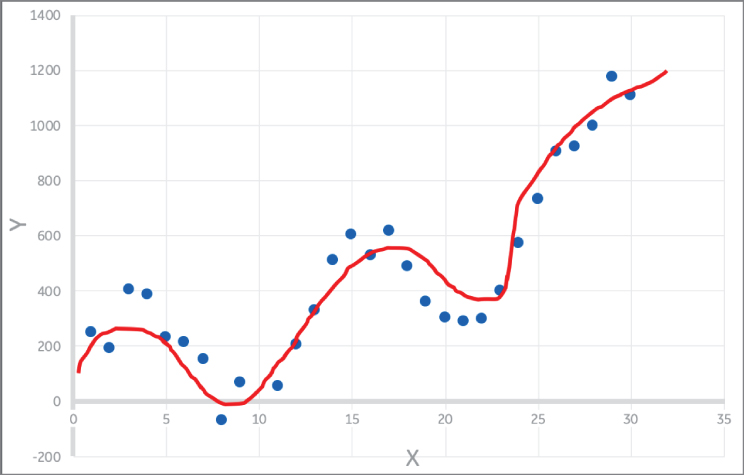
Figure 2.28: A good fit and well‐trained model!
The other option sometimes used by data scientists is to use a linear model but be aware of the bias errors and try to compensate for them using some domain knowledge of the problem. For example, in Figure 2.26, if we know that for lower values of X (say X < 25), the predicted Y values are higher than the actual values on average by 10%. And for higher values of X (say X > 25) the predicted values tend to be 10% lower than the ones expected. This is a non‐linear relationship our linear model cannot be expected to learn. However, we could put a rule of thumb or empirical factor in our calculation to add 10% of Y for predictions where X < 25 and subtract 10% of Y where X > 25. This adjustment will get us closer to the actual prediction, but involves some domain knowledge.
However, as your features increase and dataset gets more complex—particularly unstructured data like images, text, and audio—you will need to start evaluating more complex models that fit the data better and capture all the non‐linearities. This is the beginning of a huge field inside Machine Learning called Deep Learning (DL). We cover DL in detail in Chapters 4 and 5.
Reinforcement Learning
And finally, a few words about Reinforcement Learning (RL). Before that let's talk about Avengers: Infinity War. As of writing this book, it's 2018 and we are still figuring how our mighty heroes will return from the infamous snap of finger by Thanos. However, let's talk about my favorite Avenger—Dr. Strange.
In the movie, just before the final battle, Dr. Strange runs in his mind 14,000,605 scenarios of how the battle will play out. He finds that out of all those scenarios there is exactly one in which the Avengers end up defeating Thanos. Now this is kind of what Reinforcement Learning does. It builds agents that work against an environment, which can simulate actions and give you results. So over time an agent takes many actions and compares results, and it finds out which actions give favorable results and which don't. It learns a policy on how to take actions that will give maximum rewards in the long term. In Dr. Strange's case, he just had a single policy that would give him the desired end goal. But when we play game of chess, there are many ways by which we can win the game.
Now you can compare this to supervised learning. There is some supervision; however, the agent learns by taking different actions through trial and error. There is no finite training set that is prepared beforehand, as is the case with Supervised Learning. Different RL algorithms use different techniques to train and learn an optimal policy that guides them to take actions against a given environment. The key to RL is that there is no fixed dataset that the algorithm learns from. Instead, RL tries to build an agent that interacts with an environment and, based on the feedback, it learns which actions to take. See Figure 2.29.
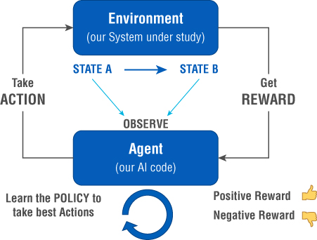
Figure 2.29: How Reinforcement Learning works
Reinforcement Learning is a special branch of ML that's probably the closest to Artificial Intelligence in its true or traditional sense. It's the process of building a system that can observe and start making decisions like humans.
RL is often considered one of the core Artificial Intelligence techniques because it is analogous to the way the human brain learns. Imagine a child learning to walk. The child keeps trying different ways to get up, establish balance, and walk. If the method is wrong, the child falls down, which is basically a negative reward or negative reinforcement. If the child is successful and takes a few steps, that's a positive reinforcement and the child's brain learns how to reproduce those exact actions. Every time the child falls, it's a negative reinforcement that tells him not to use that method. If you think closely, the child's brain does not take random movements while walking. It trains from “experience” and builds a “policy” of how to move while walking—a policy that the brain remembers for the rest of one's life.
In a similar manner, the agent in RL is given an environment to train against. It takes actions on the environment that change the state of the environment and produce a positive or negative reinforcement. These actions taken during the learning process may be taken at random but the learning process is much more effective if we consider the long‐term reward for the actions.
There are two types of RL algorithms: model‐based and model‐free. Let's look at these next.
Model‐Based RL
With this approach, we build or have a model of the environment we are building our agent to control. This model can help us answer questions like what result (new state) we will get when taking an action A on the environment in state S to get a reward R. The term model here is used for the environment rather than an ML model of the agent itself—one which we are trying to build. This is a mathematical model that captures the dynamics of the environment. Now we can use a planning algorithm to find the optimal action at any state to get the maximum reward. Basically, we can try several combinations of actions for each state and use the model to get the next state and reward and find the optimal rewarding policy. It comes down to a pure optimization problem.
In the real world, however, it's very difficult to get a true model of your environment. You have to consider the internal physics of the system you are dealing with. Then there are so many noise factors to consider. It becomes highly impractical to build a model of a system that can capture all the states, as well as their transitions and the rewards for different actions. Hence, these techniques are useful for limited and highly simplistic systems.
Let's consider a simple analogy to understand this a little better. Say that Fred is borrowing money from his friend, Anna. Anna has $200 and Fred can ask for any amount. Anna will accept or reject his ask based on some internal rule she has in her mind. Fred doesn't know what is going on inside of Anna's mind, so he doesn't know how much money to ask for.
Here we can think of Anna as our environment E. The state S of environment E is defined by a single variable—the amount of money Anna has. The initial state is that Anna has $200 with her, that is s0 = 200. Fred is our RL agent who takes an action A on the environment E. The action in this case is asking for a certain amount of money. Based on the amount of money he asks for, Anna will provide a reward R, which may be positive (accepts the ask) or negative (rejects the ask). So, our job is to figure out how much money Fred can ask Anna for, without her saying no. Figure 2.30 shows this concept.

Figure 2.30: A simple analogy for Reinforcement Learning
Model‐based RL is where we know the internal dynamics of our environment. In this example, if we know what Anna is thinking and how much money she is willing to part with, we have a simple solution to how much we should ask her for. Say Anna feels that as long as she has at least $100, then she is good. Fred can ask for up to $100 and she will most likely say yes. Here we have the environment E modeled and we know its internal workings. It's a highly simplified example, but the bottom line is that we know enough about the environment E to influence our action A and find a simple solution.
However, the real world is not so simple. There are many variables and constraints to consider as well as factors affecting how the environment behaves. It is very difficult to find the right model of the environment.
Consider a real‐world example of driving a car. We want an agent that controls the throttle position and braking so that we can drive from point A to point B. There are too many variables involved. We have to consider the dynamics of the actual car and its components like engine, brakes, throttle, etc. We have to consider wind resistance and ground friction. We have to consider safety features like spotting pedestrians and other vehicles and avoiding them. You can see how quickly this problem becomes big and it's almost impossible to accurately model such a complex environment. Hence, we need an alternate means of building our agents other than using deterministic models. That is where model‐free RL agents come into play. In fact, model‐free agents are the most popular RL methods for practical applications.
Model‐Free RL
In this case, we don't have a model of the environment. Rather we take a trial‐and‐error approach to determine the patterns for how the environment behaves. We run trials on the real system or a simulator and observe the results and learn from these observations. Through trial and error, our agent learns the patterns of actions that maximize rewards for particular states.
Let's consider an example of this approach with our friends Fred and Anna. Without any knowledge of how Anna decides on giving money out, Fred is left with no option but to try out a few requests, as shown in Figure 2.31.

Figure 2.31: Learning from reinforcements received from the environment
You can see that since Fred does not know what Anna is thinking—or the agent does not know the model of the environment—he keeps taking actions and tries to understand how Anna will react. He initially starts asking for small amounts, such as $20 and $40, and increases his ask until he gets rejected. After a rejection, he makes his ask smaller until he gets acceptance again. He also tries a new approach where he returns $20 and asks for it so that he knows how much Anna will give away.
This is the process of learning a policy that Fred is going through. The policy is what will drive his actions and, through this trial‐and‐error approach, Fred or our agent learns a good action‐making policy. The different RL algorithms like SARSA, Q‐Learning, and Deep Q Networks (DQN) take different approaches to analyzing the data and learning a good policy. The key thing that affects how an algorithm learns is how it strikes a balance between exploitation and exploration. Let's look at this in some detail:
- Exploitation means focusing on the current positive reinforcement and continuing actions along the same policy. So, if Fred got a positive reinforcement when he asked for $40 and then a negative response when he asked for $50, he can learn that as a policy and stop right there. From here, he can assume that Anna will not part with anything more than $140. Now he can keep exploiting this further by returning and borrowing the same amounts by following a strict policy that Anna's net has to be above $140. In some problems, exploitation may serve as a good strategy, especially when you arrive at a good solution immediately. However, in this case you can see that it is not.
- Exploration is when you deviate from the current policy and try something new. After being rejected for $50, Fred explores the environment further and asks for a lower amount, $30. This time he gets acceptance so the exploration approach worked. Now he can keep exploring further and try to arrive at a better policy. Again, we see that the final policy he learns in Figure 2.31 is not optimal. He could try to borrow $10 more after Anna's net reaches $110 and it will work.
RL algorithms may use different types of policies to determine the right action for the agent based on the state. For example, a random policy will have the agent take random actions. In this case, Fred will keep borrowing and returning random amounts of money until he learns the threshold amount beyond which Anna won't lend. Another policy may be a greedy policy, where Fred keeps asking for more money and chooses actions that get him the most immediate rewards.
This is how model‐free RL works. The agent tries several exploration and exploitation strategies to find an optimal policy, which can be used to take further actions. Let's next discuss a couple of the most popular RL model‐free algorithms used in practice—Q‐Learning and DQN.
Q‐Learning
The idea of Q‐Learning is to choose a policy that maximizes long‐term rewards. The concept here is to use a calculation, called the Q‐Value, that measures the long‐term reward achieved by taking a particular action when the environment is at a particular state. Hence, the Q‐Learning table, or Q‐Table, has a number of rows equal to the number of possible states and a number of columns for all the possible actions. It is usually initialized with all zero values. The cells with unrelated states and actions remain at zero.
Now we run the training or learning process, where we run each trial from start to end and find the rewards collected. For each trial, we calculate the Q‐Value for each state‐action combination using an equation called the Bellman equation. Figure 2.32 shows this Bellman equation. We will not go into details on the equation here, but I do provide references at end of the book for it. The idea is that the Bellman equation helps calculate a long‐term reward for that state‐action combination based on the results of that trial. Since this is an iterative learning process, after each trial, the appropriate Q‐Value for that state‐action cell is updated.
Figure 2.32: Bellman equation for calculating long‐term rewards
Let's consider a simple example to understand this better and more practically. Say you have a problem of traveling from point S (for start) to point E (end). You can travel different paths with middle points represented by M1, M2, etc. By traveling each path, you get a reward represented by a number. Now you have to find an optimal path to travel to maximize your rewards. This problem is represented as a Markov Decision Process (MDP) in Figure 2.33. MDP shows different states and the connections representing state transitions. It also captures the rewards for each state transition.
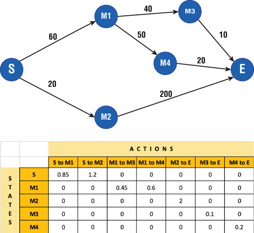
Figure 2.33: Example showing a Markov Decision Process (MDP) and a sample Q‐Learning table
The MDP shows us two possible paths from state S to E. Keep in mind that if we know this MDP beforehand, this becomes a model‐based RL problem and we can easily find the optimal path with maximum reward. We see that path S‐M2‐E is the most rewarding one. However, let's assume we don't know the MDP and through trial and error we have to find the best path. We will apply Q‐Learning. We will take each path run and calculate the Q‐Value for each state‐action pair using the Bellman equation. Over the iterations, this Q‐Value is updated in the table and you get a table like one in Figure 2.33.
Since this is a very simple problem, we only have three trials to run and calculate Q‐Values for updating the table. From the Q‐Table, we see that for each state we can choose the best action based on a maximum Q‐Value. So, we take the start state S and find the action that gives us the maximum Q‐Value. That turns out to be S‐M2 and then M2‐E gives us the best path. There we have it—S‐M2‐E is our most rewarding path, and we found this in a model‐free way.
In a real‐world problem, you'll have too many variables and state‐action combinations to consider. Imagine playing the game of chess with your friend. From the starting state where all pieces are laid out, there are almost an unimaginable number of moves and combinations of moves you can make. You need to know what your friend is thinking, anticipate her move, and make yours. Unless you are a genius like Sherlock Holmes (albeit fictitious), who can think 10–15 moves ahead of your opponent, it's pretty much impossible to consider all possible combinations.
Q‐Learning, although extremely effective, has major limitations. It works well for a finite state set that we can build in a finite table that will fit in the computer's memory. However, as the problem becomes more complex and the number of states goes from a few hundred to millions, it becomes ineffective. You can easily see that if we don't have a value in the Q‐Table for a particular state, the agent will not know what action to take.
To solve this problem, a new technique has gained popularity. It's called Deep Q Networks (DQN). Let's look at it now.
Deep Q Networks (DQN)
As we saw in the last section, Q‐Learning can handle a finite set of states. For any unseen states, it cannot predict actions to take. With real‐world systems, it is very difficult to plan for the entire state space and feed it to a Q‐Learning algorithm. Hence, we need a way to predict the Q‐Value given the state and action combination. This is done using a neural network called the Deep Q Network.
DQN trains a neural network for different combinations of state and action pairs and tries to build the Q‐Value as a dependent variable of these. DQN can now predict a Q‐Value for states that are not known to it and select the best action.
Another problem is that building a state space is often difficult. Say for a game of chess, modeling the different positions of chess pieces on the 8×8 board can be pretty challenging. A technique that is gaining popularity is feeding the images of the input medium like a chessboard and using this to decode the state. A neural network first decodes the state from an image, which is an array of pixel values. Then this decoded state is used to learn how to predict the Q‐Value.
Figure 2.34 shows how the images are fed to the network and a Q‐Value estimator is developed. The network uses convolution layers to extract features from images. These tell us where the pieces are located on the board. Then, using Supervised Learning, the prediction patterns are learned. The network starts to predict Q‐Values for different state‐action combinations. Based on highest Q‐Value, we can select that action and plan our moves.
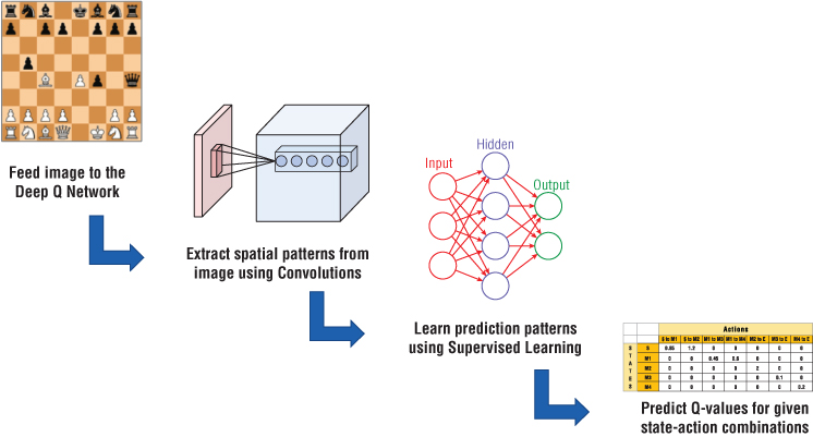
Figure 2.34: Deep Q Network to predict Q‐Values
This is an active area of research. Companies like Google's DeepMind are actively investigating new techniques for building DQNs that can solve complex problems. One of the most significant achievements of DQN has been the AlphaGo program that defeated the champion of the game Go. Go is supposed to be more complex than chess, with many more combinations, and AlphaGo was able to predict the best action for all of these.
Deep RL is a highly active and growing area. We should expect many more innovations in this space helping us reach significant milestones in fields like medical treatment, robotics, and transportation. Of course, the video game industry has been one of the front runners of using these algorithms inside games.
That's all about Reinforcement Learning for now. We will now return to general ML techniques and specifically focus on Deep Learning.
Summary
All right, that's it on Machine Learning. I hope I was able to provide you with an overview of the methods and algorithms. The code examples showed how you can apply these techniques to your datasets. I hope you can use these methods on your data and find interesting patterns.
We discussed how ML is divided into unsupervised, supervised, and Reinforcement Learning. Unsupervised ML is about finding patterns in data without knowing the results or outcomes beforehand. This includes algorithms for clustering the data, reducing the dimensions (number of features), and detecting anomalies. Supervised ML uses labeled data to build a model that can make predictions on new data. This includes classification algorithms where we predict the membership of each data point to a particular class. The other method is regression, where we predict a numerical value based on input features. We saw examples of popular algorithms in each category. Finally, we talked about Reinforcement Learning, which uses an agent that learns patterns by interacting with an environment and receiving reinforcement (rewards) for taking actions.
In the next chapter, we explore the differences between structured and unstructured data, because this difference often determines which kinds of ML algorithms we use. Then, in Chapter 4, we start looking at neural networks, which use bigger and more complex models, but will be much more effective in capturing all sorts of non‐linear patterns in your data.