4
Simulation Techniques

Simulation is an important tool for DAQ software development that permits you to test your program’s functionality without having any DAQ devices connected. This can be convenient for many reasons. Suppose your DAQ system will ultimately be running in a different city, where your testing would require travel. Unless you really like to travel on business, you will want to simulate the system near your home before the system is finished. In this book, running your program without any DAQ hardware (other than a LabVIEW-capable computer) will be termed soft simulation. To take it a step further, suppose you have the DAQ device you’ll be using, but you want to run your program without connections to the real signals. We will also cover a variety of hard simulation techniques, in which you generate real electrical signals that simulate the actual signals that your DAQ device will ultimately be handling.

It is especially nice to have a large monitor when simulating, because you can then temporarily expand the size of your front panel to accommodate the display of your simulated inputs and outputs. When you’re satisfied everything is working properly, you can delete the simulated inputs and outputs from the front panel, then shrink it to its original size.

This chapter will first discuss soft simulation, then hard simulation.

4.1 SOFT SIMULATION

Here we discuss the different categories of signals in order, as the simulation techniques in each category vary. First, analog input will be discussed, then the other forms of DAQ signals. Many concepts will be presented in this upcoming analog input section that will apply to all sections, so don’t miss it.

4.1.1 Analog Input

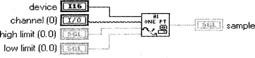
Let’s further divide analog input simulation into single-point simulation and waveform simulation. We will begin with the simplest form of analog input: single-point simulation sampling a single channel. We’ve already built such a simple VI in Chapter 3, but have another look at the DAQ portion of AI Single Point and Chart.vi, shown in Figure 4–1.

Possibly the simplest way to simulate this type of data would be to replace the DAQ function with a random number generator, as in Figure 4–2.

Figure 4–1
The DAQ portion of AI Single Point and Chart.vi.

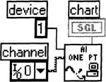
Figure 4–2
The DAQ function has been replaced with a random number generator.

This is our first example of simulating DAQ data. Unfortunately, it’s not a very powerful one, because we have no control over the data as the VI is running. Place a Horizontal Pointer Slide control on your front panel from the Controls»Numeric palette and label it Slide. We’ll use it to manually control our simulated data by wiring the DAQ portion of our block diagram as in Figure 4–3.

Figure 4–3
The numeric control lets us control our simulated data.

To generalize even further, the above example illustrates that we can use front panel controls to control our simulated DAQ data. If you were acquiring data from multiple channels, or if you were acquiring waveforms, you could use arrays on the front panel to simulate this.

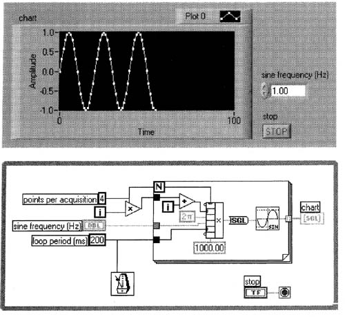
Simulating analog waveforms is usually not very difficult, provided you can define your waveform as a function of time. For example, suppose you want to simulate a 1 Hz sine wave that you’re sampling at 20 Hz, and your acquisition loop is running at 5 Hz, so you would have 4 data points per iteration of your LabVIEW loop.

Figure 4–4a shows a VI that will generate just such a 4-point section of a simulated pure sine wave per iteration of the White Loop.

Build this VI, as we will use it again in Chapter 6. The Functions»Numeric»Conversion»To Single Precision Float function is used, as this is the data type used by real DAQ functions. Use a Waveform Chart on the front panel, turn autoscaling on for the y-axis, and set the point style as shown. For simplicity and clarity, we are sending an array of numerics rather than the Waveform data type to the chart, and we are not scaling the x-axis to seconds or milliseconds—so the units seen simulate 1/20 of a second.

Figure 4–4a
This VI simulates continuous analog acquisition.

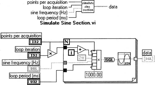
If you arrange the block diagram items as shown in Figure 4–4a, you can easily select the For Loop, the Multiply function, and the wires in between to create the subVI seen in Figure 4–4b (use Edit»Create SubVI with those items selected). Save this subVI as Simulate Sine Section.vi. The subVI should look like Figure 4–4c; if you need to rearrange its terminals through its connector pane, take care to make the right connections! Run the VI to verify that a sine wave is being drawn on the chart four points at a time. Finally, save the calling VI as Simulate AI Waveform, vi.

Figure 4–b
The new block diagram of Simulate AI Waveform. vi is shown with its new subVI Simulate Sine Section.vi.

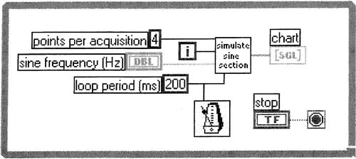
Figure 4–4c
This should be your terminal pattern and block diagram of Simulate Sine Section. vi.

4.1.2 Analog Output

Analog output simulation techniques are very similar to analog input simulation techniques. Rather than passing the data to a real DAQ function, pass it to a front panel indicator of your choice so you can monitor this value. Charts are especially useful for this because they show a history of data, unlike other indicators.

For analog output simulation, you may want to dedicate a numeric global variable per analog output line, since like real DAQ hardware, a global variable can be accessed from any VI. Heed my warnings in Chapter 1, Section 1.14.3 concerning globals, though.

4.1.3 Digital I/O

Digital I/O simulation is also very similar to analog I/O, except you generally use Booleans or integers to simulate your data, depending on whether your program operates on digital lines or digital ports, respectively.

For digital output simulation, as with analog output simulation, you may want to dedicate a Boolean or integer global variable per digital output line or port.

4.1.4 Counters

The heart of a counter is an N-bit integer, also called a register. For counting purposes, such an N-bit register can most easily be simulated with an unsigned N-bit integer global variable. Suppose you are simulating a 16-bit counter. You could create a VI that doesn’t directly correspond to any DAQ VI, but rather simulates M digital pulses physically coming into your counter. Figure 4–5 is an example of such a VI.

Figure 4–5
An example of a VI that simulates M digital pulses physically coming into the computer.

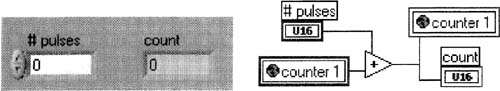
As it is the nature of unsigned N-bit integer addition to roll over to zero after the count 2^N-1 is reached, the simple structure shown in Figure 4–5 accurately simulates a 16-bit counter.

Suppose you’re trying to simulate an N-bit counter that does not conveniently have 8,16, or 32 bits, like LabVIEW’s integers do. Suppose you’re trying to simulate a 24-bit counter. In this case, you can programmatically modify the VI in Figure 4–5 with the Remainder & Quotient function, as in Figure 4–6.

Figure 4–6
A VI modified with the Remainder & Quotient function.

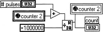
The hexadecimal number 1000000 shown in Figure 4–6 is really 2²⁴. We are using 32-bit integers, since 32 is greater than 24, whereas 16 is not.

If you’re not simply counting events, simulating timers is not always as straightforward as everything else mentioned in this section. If the timers are timing events that are slow enough, you can use LabVIEW’S timing functions, do a bit of math, and try to approximate your timer’s behavior. If the timers you’re simulating are too fast to be simulated with LabVIEW’S timing functions, you will need to come up with your own math.

4.1.5 Soft Simulation for Complicated VIs

As your DAQ Vis get more and more complex, you may find the DAQ functions buried deeply inside your code, many subVIs down. In this case, it is not always easy to wire directly from the front panel to the block diagram, so you may want to use the two following tricks: (1) Create simulated versions of all of LabVIEW’s DAQ VIs that you’re using, and (2) pass the data from your front panel simulation controls to these simulated DAQ VIs via global variables.

I will expand these two steps into many, mentioning useful details. Be patient—they’ll pay off if you need to do this.

1.   Create simulated DAQ VIs. Drop AI Sample Channel.vi from the Functions»Data Acquisition»Analog Input palette onto the block diagram of a new VI. Choose its “scaled value” version with its Select Type»Scaled Value pop up menu item. Open it and save a copy with its file name preceded by Sim, which would be Sim AI Sample Channel (scaled value).vi, in the same directory as the rest of your application’s Vis. This method saves such simulated DAQ VIs’ connector patterns, which will maintain the wiring geometry should you choose to later replace them with the original DAQ VIs. For each simulated DAQ VI, give a small unique symbol to its icon that will catch your attention at a glance. My personal preference is a small bright green s in the upper left-hand corner (probably looks like dull gray blob in this illustration): becomes .

2.   Create global variables for simulation control and for simulated data. In your new VI from the previous step, create a Boolean global variable for overall DAQ simulation control. Set this global variable to True or False at the very beginning of your overall program, and never write to it thereafter. White you have this global’s front panel open, go ahead and create another global or globals that will represent the actual data you are simulating. Since we are simulating just one number in this example (one channel, single-point acquisition), create a lone floating-point number. Your global’s front panel, for our example, should now look something like this: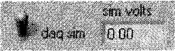

3.   Rewire simulated DAQ VIs. Go to the block diagram of your newly created simulated DAQ VI, select everything, then delete everything with the <Delete> key so that only the front panel terminals remain. My copy of LabVIEW is showing a bug that forces me to save, close, then re-open my simulated DAQ VI at this point. Next, drop the original real DAQ VI in the middle of this block diagram, and wire the corresponding terminals (see Figure 4–7).

Figure 4–7
A real DAQ VI is used as a subVI in preparation to build a simulated DAQ VI.

   As it stands, we’ve really done nothing so far; our simulated DAQ VI acts just like the real one. So let’s make it different, using your global variables from Step 2, as in Figure 4–8.

4. Use your new simulated Vis by writing to your simulated globals. The VI shown in Figure 4–9 uses our new simulated DAQ VI; we control our simulated data with the sim volts control. Note that without the Sequence Structure around the daq sim global, the loop might execute before that global is set.

Figure 4–8
Global variables are useful in building simulation VIs.

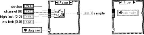
Figure 4–9
Our simulated DAQ VI in action.

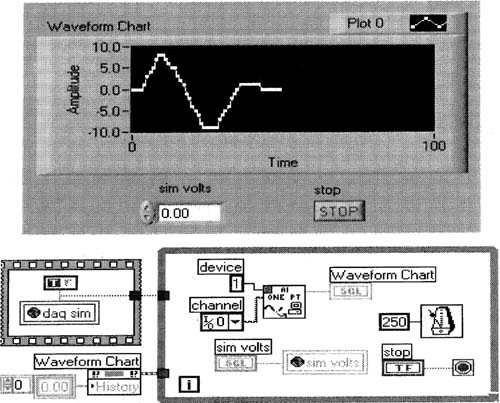
To get the chart’s plot you see in Figure 4–9, I ran the VI with sim volts at 0.00, then changed the value of the sim volts control with its up/down arrow keys during the next 20 seconds or so, then stopped the VI.

4.2 Hard Simulation

WARNING—In this section, always make sure the simulation signals’ voltages do not exceed the specs of your DAQ device.

Suppose you have your DAQ hardware, but you don’t have the real signals to which this hardware will ultimately be connected. Why not simulate these signals? As a consultant who prefers to work at home, I do this for many DAQ projects to minimize time spent onsite. Not that I don’t like my clients. I really do! Keep paying me, clients!

This section will cover real simulation signals from DAQ devices, from lab equipment and from homemade devices.

4.2.1 Simulation Signals From DAQ Devices

Luckily, many of NT’s DAQ devices are multifunction devices, meaning they have many different kinds of inputs and outputs. If you have unused output signals on any of your DAQ devices, you can use them to simulate external inputs. An analog output, when set to 0 volts or 5 volts, could simulate a TTL digital signal.

Keep in mind that many DAQ devices cannot produce accurate waveforms on their analog outputs due to the lack of DMA associated with that analog output.

Counters can be used to generate all sorts of digital signals, including square waves of varying duty cycles. LabVIEW has examples of this, some of them right on the Functions palette (such as Generate Pulse Train, vi), so I won’t bother repeating them in this book.

4.2.2 Simulation Signals From Other Lab Equipment

Companies like Agilent, Tektronix, and WaveTek make function generators whose primary purpose is generating analog voltage waveforms. As with any analog signal, they can also be used to simulate digital signals. Even the most basic function generators can generate sine waves, square waves, and triangle waves. They will also allow you to adjust the frequency, DC offset, and amplitude of these waves.

Some of the more advanced function generators allow you to simulate arbitrary waveforms that you define, should your project require nonstandard waveforms.

If you are measuring signals that are slow enough, a simple variable power supply can simulate your analog signals. Be especially careful here not to exceed the voltage limits of your DAQ device, as most variable power supplies easily exceed the basic DAQ devices’ voltage specs. A voltage divider made of two resistors is a good safety mechanism in this case, as can be seen in Chapter 2, Figure 2–19.

"Hamfests" and Internet auctions can be good sources for used lab equipment of this type. No guarantees, usually, but these sources can pan out.

4.2.3 Simulation Signals From Low-Cost, Homemade Devices

Some of the information in this section might be dated, but even so, it should give you some ideas.

I’ve put together a list of tools I personally use quite often in DAQ work:

1.   a voltmeter that can read Ohms as well (Fluke makes reliable models)

2.   small, flat-blade screwdriver

3.   22-gauge solid wire

4.   wire cutter

5.   wire stripper

6.   needle-nose pliers

7.   several test leads with tiny hook clips on either end

8.   solderless breadboard

9.   IC extractor (only if you’re using ICs, like the one shown in the breadboard in Figure 4–10)

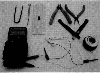
Figure 4–10 shows my own versions of these tools for assembling test circuits.

The solderless breadboard allows you to quickly assemble test circuits. I’ve put in a little DIP (Dual In-line Pin) chip just to show you how these are used, but you can easily add more common discrete components, such as resistors, capacitors, and so on. Additional helpful tools would be a DC power supply (if your DAQ device can’t provide enough current for your test circuit), a Philips screwdriver, screwdrivers with larger handles for more torque, soldering equipment, a wire stripper for very tiny wires, and a second wire stripper for very large wires. Where do you get these parts? See the Electronics Suppliers section of www.LCtechnology.com/daq-hardward.htm.

Figure 4–10
My own well-used DAQ tools—the basics.

If you need a sine waveform or other simple waveform in roughly the 20Hz to 20KHz range with a peak-to-peak magnitude of 3 volts or less, and don’t want to spend hundreds of dollars on a function generator, a common sound card will do this! See Chapter 8, Section 8.2.1 for more details.

If you want to build a homebrew circuit from scratch, Radio Shack has a couple of useful handbooks, Basic Semiconductor Circuits and Op Amp IC Circuits, both by Forest M. Mims III, published by Radio Shack, which talk about generating sine waves and square waves. Jameco sells an inexpensive function generator kit. This kit is based upon a dedicated function-generating IC, so you may want to look around and see what types of function-generating ICs exist; Digi-Key is currently a good source for these. If you only want to generate digital waveforms, simple square waves of varying duty cycles can be built from parts mentioned earlier in this paragraph, or highly complex patterns can be generated from a microcontroller (from Microchip, Motorola, and others). Microcontrollers, as fun as they are (for me), can be time-consuming to learn and use.

Low-speed digital signals can be read from or written to a computer’s parallel port. See Chapter 8, Section 8.2.2 for details.