Let's explain and implement a mean reversion strategy that relies on the Absolute Price Oscillator (APO) trading signal indicator we explored in Chapter 2, Deciphering the Markets with Technical Analysis. It will use a static constant of 10 days for the Fast EMA and a static constant of 40 days for the Slow EMA. It will perform buy trades when the APO signal value drops below -10 and perform sell trades when the APO signal value goes above +10. In addition, it will check that new trades are made at prices that are different from the last trade price to prevent overtrading. Positions are closed when the APO signal value changes sign, that is, close short positions when APO goes negative and close long positions when APO goes positive.

In addition, positions are also closed if currently open positions are profitable above a certain amount, regardless of APO values. This is used to algorithmically lock profits and initiate more positions instead of relying only on the trading signal value. Now, let's look at the implementation in the next few sections:

1. We will fetch data the same way we have done in the past. Let's fetch 4 years of GOOG data. This code will use the DataReader function from the pandas_datareader package. This function will fetch the GOOG prices from Yahoo Finance between 2014-01-2014 and 2018-01-01. If the .pkl file used to store the data on the disk is not present, the GOOG_data.pkl file will be created. By doing that, we ensure that we will use the file to fetch the GOOG data for future use:

import pandas as pd
from pandas_datareader import data

# Fetch daily data for 4 years
SYMBOL='GOOG'
start_date = '2014-01-01'
end_date = '2018-01-01'
SRC_DATA_FILENAME=SYMBOL + '_data.pkl'

try:
  data = pd.read_pickle(SRC_DATA_FILENAME)
except FileNotFoundError:
  data = data.DataReader(SYMBOL, 'yahoo', start_date, end_date)
  data.to_pickle(SRC_DATA_FILENAME)

2. Now we will define some constants and variables we will need to perform Fast and Slow EMA calculations and APO trading signal:

# Variables/constants for EMA Calculation:
NUM_PERIODS_FAST = 10 # Static time period parameter for the fast EMA
K_FAST = 2 / (NUM_PERIODS_FAST + 1) # Static smoothing factor parameter for fast EMA
ema_fast = 0
ema_fast_values = [] # we will hold fast EMA values for visualization purposes

NUM_PERIODS_SLOW = 40 # Static time period parameter for slow EMA
K_SLOW = 2 / (NUM_PERIODS_SLOW + 1) # Static smoothing factor parameter for slow EMA
ema_slow = 0
ema_slow_values = [] # we will hold slow EMA values for visualization purposes

apo_values = [] # track computed absolute price oscillator value signals

3. We will also need variables that define/control strategy trading behavior and position and PnL management:

# Variables for Trading Strategy trade, position & pnl management:
orders = [] # Container for tracking buy/sell order, +1 for buy order, -1 for sell order, 0 for no-action
positions = [] # Container for tracking positions, positive for long positions, negative for short positions, 0 for flat/no position
pnls = [] # Container for tracking total_pnls, this is the sum of closed_pnl i.e. pnls already locked in and open_pnl i.e. pnls for open-position marked to market price

last_buy_price = 0 # Price at which last buy trade was made, used to prevent over-trading at/around the same price
last_sell_price = 0 # Price at which last sell trade was made, used to prevent over-trading at/around the same price
position = 0 # Current position of the trading strategy
buy_sum_price_qty = 0 # Summation of products of buy_trade_price and buy_trade_qty for every buy Trade made since last time being flat
buy_sum_qty = 0 # Summation of buy_trade_qty for every buy Trade made since last time being flat
sell_sum_price_qty = 0 # Summation of products of sell_trade_price and sell_trade_qty for every sell Trade made since last time being flat
sell_sum_qty = 0 # Summation of sell_trade_qty for every sell Trade made since last time being flat
open_pnl = 0 # Open/Unrealized PnL marked to market
closed_pnl = 0 # Closed/Realized PnL so far

4. Finally, we clearly define the entry thresholds, the minimum price change since last trade, the minimum profit to expect per trade, and the number of shares to trade per trade:

# Constants that define strategy behavior/thresholds
APO_VALUE_FOR_BUY_ENTRY = -10 # APO trading signal value below which to enter buy-orders/long-position
APO_VALUE_FOR_SELL_ENTRY = 10 # APO trading signal value above which to enter sell-orders/short-position
MIN_PRICE_MOVE_FROM_LAST_TRADE = 10 # Minimum price change since last trade before considering trading again, this is to prevent over-trading at/around same prices
MIN_PROFIT_TO_CLOSE = 10 # Minimum Open/Unrealized profit at which to close positions and lock profits
NUM_SHARES_PER_TRADE = 10 # Number of shares to buy/sell on every trade

5. Now, let's look at the main section of the trading strategy, which has logic for the following:

• Computation/updates to Fast and Slow EMA and the APO trading signal
• Reacting to trading signals to enter long or short positions
• Reacting to trading signals, open positions, open PnLs, and market prices to close long or short positions:

close=data['Close']
for close_price in close:
  # This section updates fast and slow EMA and computes APO trading signal
  if (ema_fast == 0): # first observation
    ema_fast = close_price
    ema_slow = close_price
  else:
    ema_fast = (close_price - ema_fast) * K_FAST + ema_fast
    ema_slow = (close_price - ema_slow) * K_SLOW + ema_slow

  ema_fast_values.append(ema_fast)
  ema_slow_values.append(ema_slow)

  apo = ema_fast - ema_slow
  apo_values.append(apo)

6. The code will check for trading signals against trading parameters/thresholds and positions, to trade. We will perform a sell trade at close_price if the following conditions are met:

• The APO trading signal value is above the Sell-Entry threshold and the difference between the last trade price and current price is different enough.
• We are long (positive position) and either the APO trading signal value is at or above 0 or current position is profitable enough to lock profit:

  if ((apo > APO_VALUE_FOR_SELL_ENTRY and abs(close_price - last_sell_price) > MIN_PRICE_MOVE_FROM_LAST_TRADE) # APO above sell entry threshold, we should sell
    or
    (position > 0 and (apo >= 0 or open_pnl > MIN_PROFIT_TO_CLOSE))): # long from negative APO and APO has gone positive or position is profitable, sell to close position
    orders.append(-1) # mark the sell trade
    last_sell_price = close_price
    position -= NUM_SHARES_PER_TRADE # reduce position by the size of this trade
    sell_sum_price_qty += (close_price*NUM_SHARES_PER_TRADE) # update vwap sell-price
    sell_sum_qty += NUM_SHARES_PER_TRADE
    print( "Sell ", NUM_SHARES_PER_TRADE, " @ ", close_price, "Position: ", position )

7. We will perform a buy trade at close_price if the following conditions are met:
   the APO trading signal value is below the Buy-Entry threshold and the difference between the last trade price and current price is different enough. We are short (negative position) and either the APO trading signal value is at or below 0 or current position is profitable enough to lock profit:

  elif ((apo < APO_VALUE_FOR_BUY_ENTRY and abs(close_price - last_buy_price) > MIN_PRICE_MOVE_FROM_LAST_TRADE) # APO below buy entry threshold, we should buy
    or
    (position < 0 and (apo <= 0 or open_pnl > MIN_PROFIT_TO_CLOSE))): # short from positive APO and APO has gone negative or position is profitable, buy to close position
    orders.append(+1) # mark the buy trade
    last_buy_price = close_price
    position += NUM_SHARES_PER_TRADE # increase position by the size of this trade
    buy_sum_price_qty += (close_price*NUM_SHARES_PER_TRADE) # update the vwap buy-price
    buy_sum_qty += NUM_SHARES_PER_TRADE
    print( "Buy ", NUM_SHARES_PER_TRADE, " @ ", close_price, "Position: ", position )
  else:
    # No trade since none of the conditions were met to buy or sell
    orders.append(0)
  positions.append(position)

8. The code of the trading strategy contains logic for position/PnL management. It needs to update positions and compute open and closed PnLs when market prices change and/or trades are made causing a change in positions:

# This section updates Open/Unrealized & Closed/Realized positions
  open_pnl = 0
  if position > 0:
    if sell_sum_qty > 0: # long position and some sell trades have been made against it, close that amount based on how much was sold against this long position
      open_pnl = abs(sell_sum_qty) * (sell_sum_price_qty/sell_sum_qty - buy_sum_price_qty/buy_sum_qty)
    # mark the remaining position to market i.e. pnl would be what it would be if we closed at current price
    open_pnl += abs(sell_sum_qty - position) * (close_price - buy_sum_price_qty / buy_sum_qty)
  elif position < 0:
    if buy_sum_qty > 0: # short position and some buy trades have been made against it, close that amount based on how much was bought against this short position
      open_pnl = abs(buy_sum_qty) * (sell_sum_price_qty/sell_sum_qty - buy_sum_price_qty/buy_sum_qty)
    # mark the remaining position to market i.e. pnl would be what it would be if we closed at current price
    open_pnl += abs(buy_sum_qty - position) * (sell_sum_price_qty/sell_sum_qty - close_price)
  else:
    # flat, so update closed_pnl and reset tracking variables for positions & pnls
    closed_pnl += (sell_sum_price_qty - buy_sum_price_qty)
    buy_sum_price_qty = 0
    buy_sum_qty = 0
    sell_sum_price_qty = 0
    sell_sum_qty = 0
    last_buy_price = 0
    last_sell_price = 0

  print( "OpenPnL: ", open_pnl, " ClosedPnL: ", closed_pnl )
  pnls.append(closed_pnl + open_pnl)

9. Now we look at some Python/Matplotlib code to see how to gather the relevant results of the trading strategy such as market prices, Fast and Slow EMA values, APO values, Buy and Sell trades, Positions and PnLs achieved by the strategy over its lifetime and then plot them in a manner that gives us insight into the strategy's behavior:

# This section prepares the dataframe from the trading strategy results and visualizes the results
data = data.assign(ClosePrice=pd.Series(close, index=data.index))
data = data.assign(Fast10DayEMA=pd.Series(ema_fast_values, index=data.index))
data = data.assign(Slow40DayEMA=pd.Series(ema_slow_values, index=data.index))
data = data.assign(APO=pd.Series(apo_values, index=data.index))
data = data.assign(Trades=pd.Series(orders, index=data.index))
data = data.assign(Position=pd.Series(positions, index=data.index))
data = data.assign(Pnl=pd.Series(pnls, index=data.index))

10. Now we will add columns to the data frame with different series that we computed in the previous sections, first the Market Price and then the fast and slow EMA values. We will also have another plot for the APO trading signal value. In both plots, we will overlay buy and sell trades so we can understand when the strategy enters and exits positions:

import matplotlib.pyplot as plt

data['ClosePrice'].plot(color='blue', lw=3., legend=True)
data['Fast10DayEMA'].plot(color='y', lw=1., legend=True)
data['Slow40DayEMA'].plot(color='m', lw=1., legend=True)
plt.plot(data.loc[ data.Trades == 1 ].index, data.ClosePrice[data.Trades == 1 ], color='r', lw=0, marker='^', markersize=7, label='buy')
plt.plot(data.loc[ data.Trades == -1 ].index, data.ClosePrice[data.Trades == -1 ], color='g', lw=0, marker='v', markersize=7, label='sell')
plt.legend()
plt.show()

data['APO'].plot(color='k', lw=3., legend=True)
plt.plot(data.loc[ data.Trades == 1 ].index, data.APO[data.Trades == 1 ], color='r', lw=0, marker='^', markersize=7, label='buy')
plt.plot(data.loc[ data.Trades == -1 ].index, data.APO[data.Trades == -1 ], color='g', lw=0, marker='v', markersize=7, label='sell')
plt.axhline(y=0, lw=0.5, color='k')
for i in range( APO_VALUE_FOR_BUY_ENTRY, APO_VALUE_FOR_BUY_ENTRY*5, APO_VALUE_FOR_BUY_ENTRY ):
  plt.axhline(y=i, lw=0.5, color='r')
for i in range( APO_VALUE_FOR_SELL_ENTRY, APO_VALUE_FOR_SELL_ENTRY*5, APO_VALUE_FOR_SELL_ENTRY ):
  plt.axhline(y=i, lw=0.5, color='g')
plt.legend()
plt.show()

Let's take a look at what our trading behavior looks like, paying attention to the EMA and APO values when the trades are made. When we look at the positions and PnL plots, this will become completely clear:

In the plot, we can see where the buy and sell trades were made as the price of the Google stock change over the last 4 years, but now, let's look at what the APO trading signal values where the buy trades were made and sell trades were made. According to the design of these trading strategies, we expect sell trades when APO values are positive and expect buy trades when APO values are negative:

In the plot, we can see that a lot of sell trades are executed when APO trading signal values are positive and a lot of buy trades are executed when APO trading signal values are negative. We also observe that some buy trades are executed when APO trading signal values are positive and some sell trades are executed when APO trading signal values are negative. How do we explain that?

11. As we will see in the following code, those trades are the ones executed to close profits. Let's observe the position and PnL evolution over the lifetime of this strategy:

data['Position'].plot(color='k', lw=1., legend=True)
plt.plot(data.loc[ data.Position == 0 ].index, data.Position[ data.Position == 0 ], color='k', lw=0, marker='.', label='flat')
plt.plot(data.loc[ data.Position > 0 ].index, data.Position[ data.Position > 0 ], color='r', lw=0, marker='+', label='long')
plt.plot(data.loc[ data.Position < 0 ].index, data.Position[ data.Position < 0 ], color='g', lw=0, marker='_', label='short')
plt.axhline(y=0, lw=0.5, color='k')
for i in range( NUM_SHARES_PER_TRADE, NUM_SHARES_PER_TRADE*25, NUM_SHARES_PER_TRADE*5 ):
  plt.axhline(y=i, lw=0.5, color='r')
for i in range( -NUM_SHARES_PER_TRADE, -NUM_SHARES_PER_TRADE*25, -NUM_SHARES_PER_TRADE*5 ):
  plt.axhline(y=i, lw=0.5, color='g')
plt.legend()
plt.show()

data['Pnl'].plot(color='k', lw=1., legend=True)
plt.plot(data.loc[ data.Pnl > 0 ].index, data.Pnl[ data.Pnl > 0 ], color='g', lw=0, marker='.')
plt.plot(data.loc[ data.Pnl < 0 ].index, data.Pnl[ data.Pnl < 0 ], color='r', lw=0, marker='.')
plt.legend()
plt.show()

The code will return the following output. Let's have a look at the two charts:

From the position plot, we can see some large short positions around 2016-01, then again in 2017-07, and finally again in 2018-01. If we go back to the APO trading signal values, that is when APO values went through large patches of positive values. Finally, let's look at how the PnL evolves for this trading strategy over the course of the stock's life cycle:

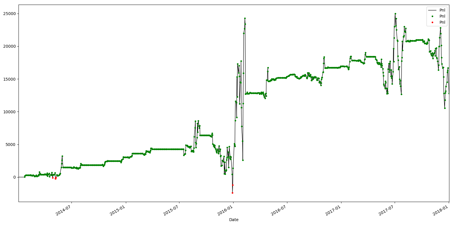
The basic mean reversion strategy makes money pretty consistently over the course of time, with some volatility in returns during 2016-01 and 2017-07, where the strategy has large positions, but finally ending around $15K, which is close to its maximum achieved PnL.