Let's implement a moving average convergence divergence signal with a fast EMA period of 10 days, a slow EMA period of 40 days, and with default smoothing factors of 2/11 and 2/41, respectively:

num_periods_fast = 10 # fast EMA time period
K_fast = 2 / (num_periods_fast + 1) # fast EMA smoothing factor
ema_fast = 0

num_periods_slow = 40 # slow EMA time period
K_slow = 2 / (num_periods_slow + 1) # slow EMA smoothing factor
ema_slow = 0

num_periods_macd = 20 # MACD EMA time period
K_macd = 2 / (num_periods_macd + 1) # MACD EMA smoothing factor
ema_macd = 0

ema_fast_values = [] # track fast EMA values for visualization purposes
ema_slow_values = [] # track slow EMA values for visualization purposes
macd_values = [] # track MACD values for visualization purposes
macd_signal_values = [] # MACD EMA values tracker

macd_histogram_values = [] # MACD - MACD-EMA

for close_price in close:
 if (ema_fast == 0): # first observation
   ema_fast = close_price
   ema_slow = close_price
 else:
   ema_fast = (close_price - ema_fast) * K_fast + ema_fast
   ema_slow = (close_price - ema_slow) * K_slow + ema_slow

 ema_fast_values.append(ema_fast)
 ema_slow_values.append(ema_slow)
 macd = ema_fast - ema_slow # MACD is fast_MA - slow_EMA

 if ema_macd == 0:
   ema_macd = macd
 else:
   ema_macd = (macd - ema_macd) * K_slow + ema_macd # signal is EMA of MACD values

 macd_values.append(macd)
 macd_signal_values.append(ema_macd)
 macd_histogram_values.append(macd - ema_macd)

In the preceding code, the following applies:

•  The  time period used a period of 20 days and a default smoothing factor of 2/21.
• We also computed a  value (- ).

Let's look at the code to plot and visualize the different signals and see what we can understand from it:

goog_data = goog_data.assign(ClosePrice=pd.Series(close, index=goog_data.index))
goog_data = goog_data.assign(FastExponential10DayMovingAverage=pd.Series(ema_fast_values, index=goog_data.index))
goog_data = goog_data.assign(SlowExponential40DayMovingAverage=pd.Series(ema_slow_values, index=goog_data.index))
goog_data = goog_data.assign(MovingAverageConvergenceDivergence=pd.Series(macd_values, index=goog_data.index))
goog_data = goog_data.assign(Exponential20DayMovingAverageOfMACD=pd.Series(macd_signal_values, index=goog_data.index))
goog_data = goog_data.assign(MACDHistorgram=pd.Series(macd_historgram_values, index=goog_data.index))
close_price = goog_data['ClosePrice']
ema_f = goog_data['FastExponential10DayMovingAverage']
ema_s = goog_data['SlowExponential40DayMovingAverage']
macd = goog_data['MovingAverageConvergenceDivergence']
ema_macd = goog_data['Exponential20DayMovingAverageOfMACD']
macd_histogram = goog_data['MACDHistorgram']

import matplotlib.pyplot as plt

fig = plt.figure()
ax1 = fig.add_subplot(311, ylabel='Google price in $')
close_price.plot(ax=ax1, color='g', lw=2., legend=True)
ema_f.plot(ax=ax1, color='b', lw=2., legend=True)
ema_s.plot(ax=ax1, color='r', lw=2., legend=True)
ax2 = fig.add_subplot(312, ylabel='MACD')
macd.plot(ax=ax2, color='black', lw=2., legend=True)
ema_macd.plot(ax=ax2, color='g', lw=2., legend=True)s
ax3 = fig.add_subplot(313, ylabel='MACD')
macd_histogram.plot(ax=ax3, color='r', kind='bar', legend=True, use_index=False)
plt.show()

The preceding code will return the following output. Let's have a look at the plot:

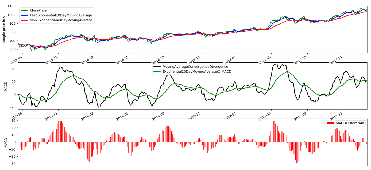
The MACD signal is very similar to the APO, as we expected, but now, in addition, the  is an additional smoothing factor on top of raw values to capture lasting trending periods by smoothing out the noise of raw  values. Finally, the , which is the difference in the two series, captures (a) the time period when the trend is starting or reversion, and (b) the magnitude of lasting trends when  values stay positive or negative after reversing signs.