In trading, the price we receive is a collection of data points at constant time intervals called time series. They are time dependent and can have increasing or decreasing trends and seasonality trends, in other words, variations specific to a particular time frame. Like any other retail products, financial products follow trends and seasonality during different seasons. There are multiple seasonality effects: weekend, monthly, and holidays.

In this section, we will use the GOOG data from 2001 to 2018 to study price variations based on the months.

1. We will write the code to regroup the data by months, calculate and return the monthly returns, and then compare these returns in a histogram. We will observe that GOOG has a higher return in October:

import pandas as pd
import matplotlib.pyplot as plt
from pandas_datareader import data

start_date = '2001-01-01'
end_date = '2018-01-01'
SRC_DATA_FILENAME='goog_data_large.pkl'

try:
  goog_data = pd.read_pickle(SRC_DATA_FILENAME)
  print('File data found...reading GOOG data')
except FileNotFoundError:
  print('File not found...downloading the GOOG data')
  goog_data = data.DataReader('GOOG', 'yahoo', start_date, end_date)
  goog_data.to_pickle(SRC_DATA_FILENAME)

goog_monthly_return = goog_data['Adj Close'].pct_change().groupby(
  [goog_data['Adj Close'].index.year,
   goog_data['Adj Close'].index.month]).mean()
goog_montly_return_list=[]

for i in range(len(goog_monthly_return)):
  goog_montly_return_list.append
      ({'month':goog_monthly_return.index[i][1],
        'monthly_return': goog_monthly_return[i]})

goog_montly_return_list=pd.DataFrame(goog_montly_return_list,
                                   columns=('month','monthly_return'))
goog_montly_return_list.boxplot(column='monthly_return', by='month')

ax = plt.gca()
labels = [item.get_text() for item in ax.get_xticklabels()]
labels=['Jan','Feb','Mar','Apr','May','Jun',
      'Jul','Aug','Sep','Oct','Nov','Dec']
ax.set_xticklabels(labels)
ax.set_ylabel('GOOG return')
plt.tick_params(axis='both', which='major', labelsize=7)
plt.title("GOOG Monthly return 2001-2018")
plt.suptitle("")
plt.show()

The preceding code will return the following output. The following screenshot represents the GOOG monthly return:

In this screenshot, we observe that there are repetitive patterns. The month of October is the month when the return seems to be the highest, unlike November, where we observe a drop in the return.

2. Since it is a time series, we will study the stationary (mean, variance remain constant over time). In the following code, we will check this property because the following time series models work on the assumption that time series are stationary:

• Constant mean
• Constant variance
• Time-independent autocovariance

# Displaying rolling statistics
def plot_rolling_statistics_ts(ts, titletext,ytext, window_size=12):
  ts.plot(color='red', label='Original', lw=0.5)
  ts.rolling(window_size).mean().plot(
          color='blue',label='Rolling Mean')
  ts.rolling(window_size).std().plot(
          color='black', label='Rolling Std')

  plt.legend(loc='best')
  plt.ylabel(ytext)
  plt.title(titletext)
  plt.show(block=False)

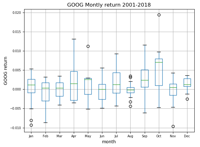
plot_rolling_statistics_ts(goog_monthly_return[1:],'GOOG prices rolling mean and standard deviation','Monthly return')

plot_rolling_statistics_ts(goog_data['Adj Close'],'GOOG prices rolling mean and standard deviation','Daily prices',365)

The preceding code will return the following two charts, where we will compare the difference using two different time series.

• One shows the GOOG daily prices, and the other one shows the GOOG monthly return.
• We observe that the rolling average and rolling variance are not constant when using the daily prices instead of using the daily return.
• This means that the first time series representing the daily prices is not stationary. Therefore, we will need to make this time series stationary.
• The non-stationary for a time series can generally be attributed to two factors: trend and seasonality.

The following plot shows GOOG daily prices:

When observing the plot of the GOOG daily prices, the following can be stated:

• We can see that the price is growing over time; this is a trend.
• The wave effect we are observing on the GOOG daily prices comes from seasonality.
• When we make a time series stationary, we remove the trend and seasonality by modeling and removing them from the initial data.
• Once we find a model predicting future values for the data without seasonality and trend, we can apply back the seasonality and trend values to get the actual forecasted data.

The following plot shows the GOOG monthly return:

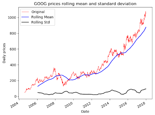
For the data using the GOOG daily prices, we can just remove the trend by subtracting the moving average from the daily prices in order to obtain the following screenshot:

• We can now observe the trend disappeared.
• Additionally, we also want to remove seasonality; for that, we can apply differentiation.
• For the differentiation, we will calculate the difference between two consecutive days; we will then use the difference as data points.

3. To confirm our observation, in the code, we use the popular statistical test: the augmented Dickey-Fuller test:

• This determines the presence of a unit root in time series.
• If a unit root is present, the time series is not stationary.
• The null hypothesis of this test is that the series has a unit root.
• If we reject the null hypothesis, this means that we don't find a unit root.
• If we fail to reject the null hypothesis, we can say that the time series is non-stationary:

def test_stationarity(timeseries):
  print('Results of Dickey-Fuller Test:')
  dftest = adfuller(timeseries[1:], autolag='AIC')
  dfoutput = pd.Series(dftest[0:4], index=['Test Statistic', 'p-value', '#Lags Used', 'Number of Observations Used'])
  print (dfoutput)

test_stationarity(goog_data['Adj Close'])

4. This test returns a p-value of 0.99. Therefore, the time series is not stationary. Let's have a look at the test:

test_stationarity(goog_monthly_return[1:])

This test returns a p-value of less than 0.05. Therefore, we cannot say that the time series is not stationary. We recommend using daily returns when studying financial products. In the example of stationary, we could observe that no transformation is needed.

5. The last step of the time series analysis is to forecast the time series. We have two possible scenarios:

• A strictly stationary series without dependencies among values. We can use a regular linear regression to forecast values.
• A series with dependencies among values. We will be forced to use other statistical models. In this chapter, we chose to focus on using the Auto-Regression Integrated Moving Averages (ARIMA) model. This model has three parameters:
  • Autoregressive (AR) term (p)—lags of dependent variables. Example for 3, the predictors for x(t) is x(t-1) + x(t-2) + x(t-3).
  • Moving average (MA) term (q)—lags for errors in prediction. Example for 3, the predictor for x(t) is e(t-1) + e(t-2) + e(t-3), where e(i) is the difference between the moving average value and the actual value.
  • Differentiation (d)— This is the d number of occasions where we apply differentiation between values, as was explained when we studied the GOOG daily price. If d=1, we proceed with the difference between two consecutive values.

The parameter values for AR(p) and MA(q) can be respectively found by using the autocorrelation function (ACF) and the partial autocorrelation function (PACF):

from statsmodels.graphics.tsaplots import plot_acf
from statsmodels.graphics.tsaplots import plot_pacf
from matplotlib import pyplot

pyplot.figure()
pyplot.subplot(211)
plot_acf(goog_monthly_return[1:], ax=pyplot.gca(),lags=10)

pyplot.subplot(212)
plot_pacf(goog_monthly_return[1:], ax=pyplot.gca(),lags=10)

pyplot.show()

Now, let's have a look at the output of the code:

When we observe the two preceding diagrams, we can draw the confidence interval on either side of 0. We will use this confidence interval to determine the parameter values for the AR(p) and MA(q).

• q: The lag value is q=1 when the ACF plot crosses the upper confidence interval for the first time.
• p: The lag value is p=1 when the PACF chart crosses the upper confidence interval for the first time.

6. These two graphs suggest using q=1 and p=1. We will apply the ARIMA model in the following code:

from statsmodels.tsa.arima_model import ARIMA

model = ARIMA(goog_monthly_return[1:], order=(2, 0, 2))

fitted_results = model.fit()

goog_monthly_return[1:].plot()

fitted_results.fittedvalues.plot(color='red')

plt.show()

As shown in the code, we applied the ARIMA model to the time series and it is representing the monthly return.