Chapter 1. Problem solving
What is an Algorithm?
Explaining how an algorithm works is like telling a story. Each algorithm introduces some novel concept or innovation that improves over ordinary solutions. In this chapter we explore several solutions to a simple problem to explain the factors that affect an algorithm’s performance. Along the way I will introduce techniques used to analyze an algorithm’s performance, independent of its implementation, though I will always provide empirical evidence from actual implementations.
Tip
An algorithm is a step-by-step problem solving method implemented as a computer program that returns a correct answer in a predictable amount of time. The study of algorithms is concerned with both correctness (will this algorithm work for all input?) and performance (is this the most efficient way to solve this problem?).
Let’s walk through an example of a problem solving method to see what this looks like in practice. What if you wanted to find the largest value in an unordered list? Each Python list in Figure 1-1 is a problem instance, that is, the input processed by an algorithm (shown as a cylinder); the correct answer appears on the right. How is this algorithm implemented? How would it perform on different problem instances? Can you predict the time needed to find the largest value in a list of one million elements?

Figure 1-1. Three different problem instances processed by an algorithm
An algorithm is more than just a problem solving method; the program also
needs to complete in a predictable amount of time. The built-in Python
function max() already solves this problem. However, it can be hard to
predict an algorithm’s performance on problem instances containing random
data, so it’s worth identifying problem instances whose structure is
regular. Table 1-1 shows the results of timing max() on two
kinds of problem instances of size N, one where the list contains ascending
integers and one where the list contains descending integers. You can
execute the ch01.timing program to generate this table. While you will
get different values in the table, based on the configuration of your
computing system, you can verify the following two statements:
-
The timing for
max()on ascending values is always slower than on descending values once N is large enough; and -
As N increases ten-fold in subsequent rows, the corresponding time for
max()also appears to increase ten-fold, with some deviation to be expected from live performance trials.
For this problem, the maximum value is returned and the input is unchanged. In some cases, the algorithm updates the problem instance directly instead of computing a new value — for example, sorting a list of values as you will see in chapter five. Throughout this book, we use N to represent the size of a problem instance.
| N | Ascending values | Descending values |
|---|---|---|
100 |
|
|
1,000 |
|
|
10,000 |
|
|
100,000 |
|
|
1,000,000 |
|
|
When it comes to timing, the key points are that:
-
You can’t predict in advance the value of
T(1,000), that is, the time required by the algorithm to solve a problem instance of size1,000, because computing platforms vary and there may be different programming languages used; however, -
Once you empirically determine
T(1,000), you can predictT(100,000), that is, the time to solve a problem instance one hundred times larger.
Now that we’ve walked through a sample algorithm, it’s important to understand the concept of correctness, whether this algorithm will work for all inputs. We will spend more time in chapter two explaining how to compare the behavior of different algorithms that solve the exact same problem. While the mathematics of algorithms can get quite tricky, I will provide specific examples to always connect the abstract concepts with real-world problems.
The Almighty Array
The standard way to judge the efficiency of an algorithm is to count how
many computing operations it requires. But this is exceptionally hard to
do! Computers have a central processing unit (CPU) that executes machine
instructions that perform mathematical computations (like add and
multiply), assign values to CPU registers, and compare two values with each
other. Modern programming languages are either compiled into machine
instructions (like C or C++) or an intermediate byte code representation
(like Python and Java). The Python interpreter (which is itself a C
program) executes the byte code and built-in functions, such as min() and
max(), are implemented in C and ultimately compiled into machine
instructions for execution. Whew! That is a lot to take in!
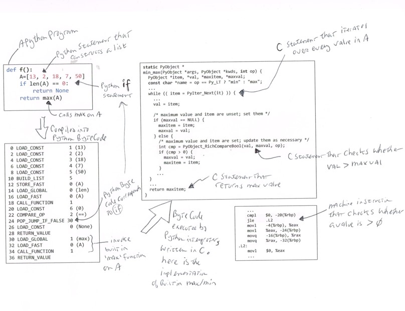
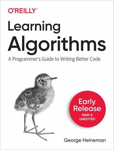
Figure 1-2. Counting operations or instructions is complicated
In Figure 1-2, the Python function, f(), is compiled
into 19 byte code instructions. This byte code is executed by a Python
interpreter, written in C, which includes the implementation of the
built-in max() function. This interpreter is itself compiled into machine
instructions, and the jle (“jump less than or equal”) machine instruction
corresponds to the C program statement that compares whether cmp > 0.
It is nearly impossible to count the total number of executed machine
instructions for an algorithm, not to mention that modern day CPUs can
execute billions of instructions per second! Instead, we will count the
number of times a key operation is invoked for each algorithm, which
could be “the number of times two elements in a list are compared with each
other” or “how many times a function is called.” In this discussion of
max(), the key operation is “how many times the less-than (<) operator
is invoked.” We will expand on this counting principle in chapter two.
At the end of every chapter in the book, I pose challenge problems that give you a chance to put your new knowledge to the test. I encourage you to try these on your own before you review my sample solutions.
Now is a good time to lift up the hood on the max algorithm to see why it
behaves the way it does. All algorithms in this chapter will use Python.
Finding the largest value in an arbitrary list
Consider the following (flawed) Python implementation that attempts to find
the largest value in an arbitrary list by comparing each value in A
against my_max, updating my_max as needed when larger values are found.
defflawed(A):my_max=0forvinA:ifmy_max<v:my_max=vreturnmy_max

my_maxis a variable that holds the maximum value; heremy_maxis initialized to0.
The for loop defines a variable
vthat iterates over each element inA. The if statement executes once for each value,v.
Update
my_maxifvis larger.
Central to this solution is the less-than operator (<) that compares two numbers to determine whether a value is smaller than another.
>>> p = [1, 5, 2, 9, 3, 4]
>>> flawed(p)
9
flawed correctly determines the largest value for p, invoking the
less-than operator six times, once for each of its values. flawed
invokes the less-than operator N times on a problem instance of size
N. In Figure 1-3, as v takes on successive values
from A, you can see that my_max is updated three times to determine the
largest value in A.
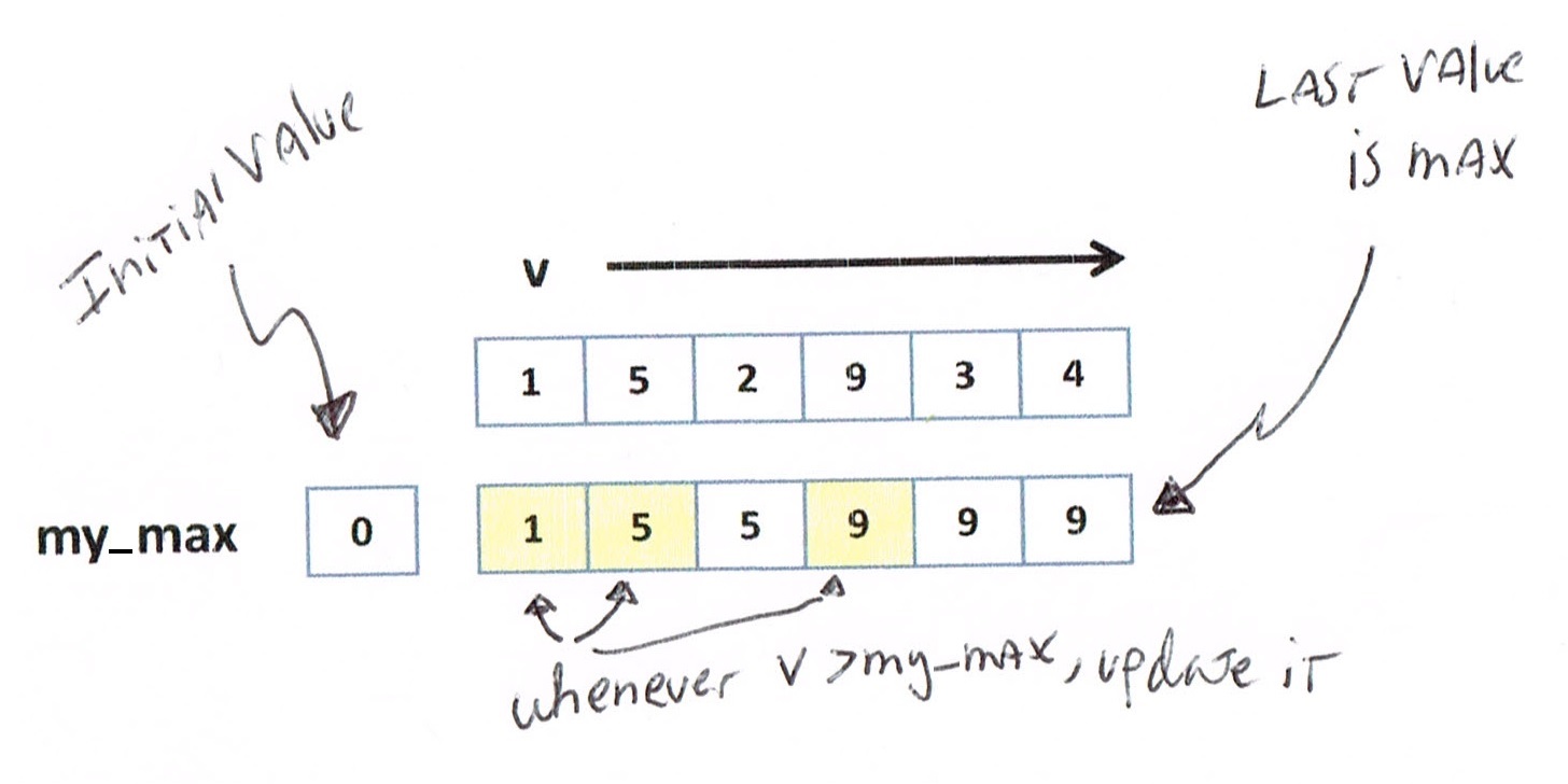
Figure 1-3. Visualizing the execution of flawed
This implementation is flawed because it assumes that at least one value in
A is greater than 0. Computing flawed([-5,-3,-11]) returns 0, which
is incorrect. One common fix is to initialize my_max to the smallest
possible value, such as my_max = float('-inf'). This approach is still
flawed since it would return this value on an empty problem instance. Let’s
fix this defect now.
Counting key operations
Since the largest value must be an element in A, largest selects the
first element of A as my_max, checking other elements to see if any is
larger.
deflargest(A):my_max=A[0]foridxinrange(1,len(A)):ifmy_max<A[idx]:my_max=A[idx]returnmy_max
Set
my_maxto the first element inA, found at index position 0.idxtakes on integer values from 1 up to, but not including,len(A).Update
my_maxif the element inAat positionidxis larger.
When given a non-empty list, largest returns the largest element in the
list. Now that we have a correct Python implementation of our algorithm,
can you determine how many times less-than is invoked in this new
algorithm? Right! N–1 times. We have fixed the flaw in the algorithm and
improved its performance (admittedly, by just a tiny bit).
Why is it important to count the uses of less-than? This is the key operation used when comparing two elements. All other program statements (such as for or while loops) are arbitrary choices during implementation, based on the program language used. We will expand on this idea in the next chapter, but for now counting key operations is sufficient.
Models can predict algorithm performance
What if someone shows you a different algorithm for this same problem? How
would you determine which one to select? Consider the following alternate
algorithm that repeatedly checks each element in the list to see if it is
larger than all other elements in the same list. Will this algorithm
return the correct result? How many times does it invoke less-than on a
problem of size N?
defalternate(A):forvinA:none_greater_than_v=TrueforxinA:ifv<x:none_greater_than_v=Falsebreakifnone_greater_than_v:returnvreturnNone
When iterating over each
v, assume it could be the largest.If
vis smaller than another element,x, stop and record thatvis not greatest.If
none_greater_than_vistrue, returnvsince it is maximum.
This final statement is here in case
Ais an empty list.
alternate attempts to find a value, v, in A such that no other value,
x, in A is greater. The implementation uses two nested for loops.
This time it’s not so simple to compute how many times less-than is
invoked, because the inner for loop stops as soon as an x is found that
is greater than v. Also, the outer for loop stops once the maximum
value is found. Figure 1-4 visualizes executing
alternate on our list example.

Figure 1-4. Visualizing the execution of alternate
For this problem-instance, less-than is invoked 14 times. But you can
see that this total count depends on the specific values in the list
A. What if the values were in a different order? Can you think of an
arrangement of values that requires the least number of less-than
invocations? Such a problem instance would be considered a best case for
alternate. For example, if the first value in A is the largest of the N
values, then the total number of calls to less-than is always N.
Tip
Best Case — a problem instance of size N that requires the least amount of work performed by the algorithm.
Worst Case — a problem instance of size N that demands the most amount of work.
Let’s try to identify a worst case problem instance for alternate that
requires the most number of calls to less-than. More than just ensuring
that the largest value is the last value in A, in a worst case problem
instance for alternate, the values in A must appear in ascending order.
Figure 1-5 shows a best case on the left (p
= [9,5,2,1,3,4]) and a worst case on the right (p = [1,2,3,4,5,9]).
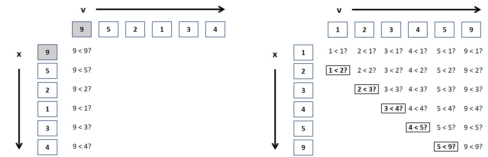
Figure 1-5. Visualizing the execution of alternate on best and worst cases
In the best case, there are six calls to less-than; if there were N
values in a best case, then the total number of invocations to
less-than would be N. It’s a bit more complicated for the worst
case. In Figure 1-5 you can see there are a total of
26 calls to less-than when the list of N values is in ascending sorted
order. With a little bit of mathematics, I can show that for N elements,
this will always be (N2 + 3*N - 2)/2. The following table
presents empirical evidence on largest and alternate on worst case
problem instances of size N.
| N | Largest (# less-than) | Alternate (# less-than) | Largest (time in ms) | Alternate (time in ms) |
|---|---|---|---|---|
8 |
|
|
|
|
16 |
|
|
|
|
32 |
|
|
|
|
64 |
|
|
|
|
128 |
|
|
|
|
256 |
|
|
|
|
512 |
|
|
|
|
1024 |
|
|
|
|
2048 |
|
|
|
|
For small problem instances, it doesn’t seem all that bad, but as we double
the size of the problem instances, you can see that the number of
less-than invocations for alternate nearly quadruples, far surpassing
the count for largest. The next two columns in
Table 1-2 show the performance of these two
implementations on 100 random trials of problem instances of size N. The
completion time for alternate quadruples as well.
Note
There are many different approaches to evaluate runtime performance of a target algorithm. In this book, I execute repeated random problem instances of size N and measure the time (in milliseconds) required by an algorithm to process each one. From this set of runs, I select the quickest completion time (i.e., the smallest). This is preferable to simply averaging the total running time over all runs, since that might skew the results.
Counting the number of less-than invocations helps explain the behaviors
of largest and alternate. As N doubles, the number of calls to
less-than doubles for largest but quadruples for alternate. This
behavior is consistent as N increases and you can use this information to
predict the run-time performance of these two algorithms on larger-sized
problems.
Congratulations! You’ve just performed a key step in algorithmic analysis –
judging the relative performance of two algorithms by counting the number
of times a key operation is performed. You can certainly go and implement
both variations and measure their respective elapsed times on problems
instances that double in size; but it actually isn’t necessary since the
model predicts this behavior, and confirms that largest is the more
efficient algorithm of the two.
Table 1-3 shows that largest is always
significantly slower than max(), typically four times slower. Ultimately
the reason is that Python is an interpreted language, and built-in
functions, such as max(), will always outperform an identical Python
implementation. What you should observe is that in all cases, as N doubles,
the corresponding performance of largest and max - for both best case
and worst case - also doubles.
| N | Largest Worst Case | Max Worst Case | Largest Best Case | Max Best Case |
|---|---|---|---|---|
4,096 |
|
|
|
|
8,192 |
|
|
|
|
16,384 |
|
|
|
|
32,768 |
|
|
|
|
65,536 |
|
|
|
|
131,072 |
|
|
|
|
262,144 |
|
|
|
|
524,288 |
|
|
|
|
Table 1-3 shows it is possible to predict the time required to solve problems instances of increasing size. Now let’s change the problem slightly to make it more interesting.
Find two largest values in arbitrary list
Devise an algorithm that finds the two largest values in an arbitrary
list. Perhaps you can modify the existing largest algorithm with just a
few tweaks.
Why don’t you take a stab at solving this modified problem and come back here with your solution.
deftwo_largest(A):my_max,second=A[:2]ifmy_max<second:my_max,second=second,my_maxforidxinrange(2,len(A)):ifmy_max<A[idx]:my_max,second=A[idx],my_maxelifsecond<A[idx]:second=A[idx]return(my_max,second)
Determine
my_maxandsecondof first two elements, swapping if out of order.If
A[idx]is a new max value, thenmy_maxbecomes that max value, andsecondbecomes the oldmy_max.If a value is larger than
second(but smaller thanmy_max), only updatesecond.
two_largest feels similar to largest: compute my_max and second to
be the first two elements in A, properly ordered. Then for each of the
remaining elements in A (how many? N–2, right!) if you find an A[idx]
larger than my_max, adjust both (my_max, second) otherwise check to see
whether second alone needs updating.
Counting the number of times less-than is invoked is more complicated because, once again, it depends on the values in the problem instance.
In the best case, two_largest performs the fewest less-than
invocations when if statement ![]() is true. When
is true. When
A is in ascending sorted order, the less-than at
![]() is always true, so it is invoked N–2 times;
don’t forget to add
is always true, so it is invoked N–2 times;
don’t forget to add 1 because of the use of less-than at
![]() . In the best case, therefore, you only need
N–1 invocations of less-than to determine the top two values. The
less-than at
. In the best case, therefore, you only need
N–1 invocations of less-than to determine the top two values. The
less-than at ![]() is never used in the best
case.
is never used in the best
case.
For two_largest, can you construct a worst case problem instance? Try
it yourself: it happens whenever less-than at ![]() is
is False.
I bet you can see that whenever the list A is in descending order,
two_largest requires the most uses of less-than. In particular, for the
worst case, less-than is used twice each time through the for loop,
or 1 + 2*(N–2) = 2*N–3 times. Somehow this feels right, doesn’t it? If
you need N–1 uses of less-than to find the largest value in A,
perhaps you truly do need an additional N–2 comparisons (leaving out the
largest value, of course) to also find the second largest value.
To summarize:
-
For best case,
two_largestfinds both values in N–1 uses of less-than. -
In worst case,
two_largestfinds both values in 2N–3 uses of less-than.
Note
If you determine the worst case for a particular algorithm on a given problem, perhaps a different algorithm solving the same problem could do better.
Are we done? is this the “best” algorithm to solve the problem of finding the two largest values in an arbitrary list? We can choose to prefer one algorithm over another based on a number of factors:
-
Required extra storage - Does an algorithm need to make a copy of the original problem instance?
-
Programming effort - How few lines of code must the programmer write?
-
Mutable input - Does the algorithm modify the input provided by the problem instance in place, or does it leave it alone?
-
Speed - Does an algorithm outperform the competition?
Let’s investigate three different algorithms to solve this exact same
problem, starting with two brief algorithms with no explicit less-than
usage (making it hard to know in advance how well they perform relative to
largest).
two_largest_sorting creates a new list containing the values in A in
increasing order, grabs the final two values and reverses
them. two_largest_extra_storage uses max() to find the maximum value in
A, removes it from a copy of A and then finds the max of that reduced
list to be second. Both of these algorithms require extra storage and only
work on lists with more than one value.
We can compare these algorithms against largest by their run-time
performance; but first, I want to introduce one final algorithm that uses
far fewer less-than invocations than largest, and basketball fans will
find its logic familiar.
deftwo_largest_sorting(A):returntuple(reversed(sorted(A)[-2:]))deftwo_largest_extra_storage(A):my_max=max(A)copy=list(A)copy.remove(my_max)return(my_max,max(copy))
Sort
Ato create a new list whose values are in ascending order, select the last two values, reverse their order and return as a tuple.Uses built-in
max() function to find largest.Create a copy of the original
Aand removemy_max.Return a tuple containing
my_maxand the largest value incopy.
Tournament algorithm
A single-elimination tournament consists of a number of teams competing to see who is the champion. Ideally, the number of teams is a power of 2, like 16 or 64. The tournament is built from a sequence of rounds where all remaining teams in the tournament are paired up to play a match; match losers are eliminated, while winners advance to the next round. The final team remaining is the tournament champion.
Consider the problem instance p=[3,1,4,1,5,9,2,6] with N=8
values. Figure 1-6 shows the single-elimination tournament
whose initial round consists of comparing neighboring values using
less-than, and the larger values advance in the tournament. In the Elite
Eight round, four teams are eliminated, leaving values [3, 4, 9, 6]. In
the Final Four round, the values [4, 9] advance and in the Championship
round, 9 is declared the victor.

Figure 1-6. A tournament with eight initial values
In this tournament, there are seven less-than invocations, which should
be reassuring, since this means the largest value was found with N–1 uses
of less-than, as we had discussed earlier. If you store each of these
N-1 matches, then you can quickly locate the second largest value, as I
now show.
Where can the second largest value be “hiding” once 9 is declared the
champion? Select 4 as the candidate second-largest value, since this was
the value that lost in the Championship round. But the largest value, 9,
had two earlier matches, so you must check the other two losing values –
value 6 in the Final Four round and value 5 in the Elite Eight
round. Thus the second largest value is 6.
For eight initial values, you need just 2 additional less-than
invocations – (is 4 < 6) and (is 6 < 5) – to determine that 6 is
the second largest value. Because 8=23, you need 3-1=2
comparisons. In general, for N = 2K, you need an additional K–1
comparisons, where K is the number of rounds.
When there are 8=23 initial values, the algorithm constructs a
tournament with 3 rounds. To double the number of values in the
tournament, you only need one additional round of matches; in other words,
with each new round K, you can add 2K more values. Want to find the
largest of 64 values? you only need 6 rounds.
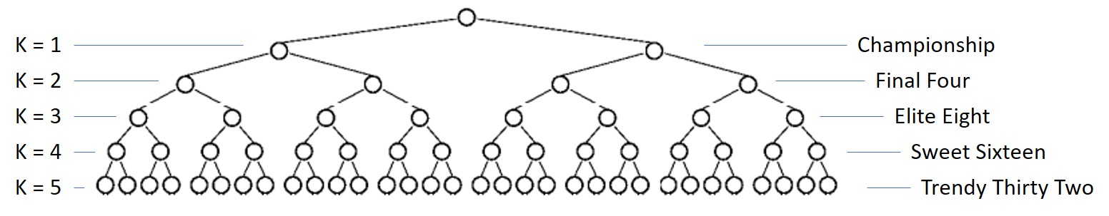
Figure 1-7. A tournament with thirty-two values
To determine the number of rounds given any N, we turn to the logarithm
function, which is the opposite of the exponent operation. With N=8
initial values, there are 3 rounds required for the tournament, since
23=8 and log2(8) = 3. In this book, and traditionally in
computer science, the log() operator is in base 2, unless otherwise
specified.
When N is a power of 2 – like 64 or 65,536 – the number of rounds in a
tournament is log(N), which means the number of extra less-than
usages is log(N)–1.
I have just sketched an algorithm to compute the largest and second largest
value in A using just N–1+log(N)–1 = N+log(N)-2 less-than invocations
for any N that is a power of 2.
Is this tournament_two algorithm practical? Will it outperform
two_largest? If you only count the number of times less-than is
invoked, tournament_two is noticeably better. two_largest requires
131,069 less-than operations on problems of size N while
tournament_two only requires 65,536 + 16 – 2 = 65,550, just about
half. But there is more to the story.
deftournament_two(A):N=len(A)winner=[None]*(N-1)loser=[None]*(N-1)prior=[-1]*(N-1)idx=0foriinrange(0,N,2):ifA[i]<A[i+1]:winner[idx]=A[i+1]loser[idx]=A[i]else:winner[idx]=A[i]loser[idx]=A[i+1]idx+=1m=0whileidx<N-1:ifwinner[m]<winner[m+1]:winner[idx]=winner[m+1]loser[idx]=winner[m]prior[idx]=m+1else:winner[idx]=winner[m]loser[idx]=winner[m+1]prior[idx]=mm+=2idx+=1largest=winner[idx-1]second=loser[idx-1]m=prior[idx-1]whilem>=0:ifsecond<loser[m]:second=loser[m]m=prior[m]return(largest,second)
Create arrays for
winnerandloservalues, and index ofpriormatches.Populate first
N/2winner/loser pairs usingN/2invocations of less-than.Pair up winners to find new winner and record
priormatch index.An additional
N/2-1invocations of less-than.
Advance
mby two to find next pair of winners. WhenidxreachesN-1,winner[idx-1]is largest.
Initial candidate for second largest, but must check all others that lost to
largestto find actual second largest.
log(N)-1additional invocations of less-than.
Table 1-4 reveals that tournament_two is almost ten
times slower than any of its competitors! Let’s record the total time it
takes to solve 100 random problem instances (of size N growing from
1,024 to 16,384). While we are at it, I will include the performance
results of two_largest_sorting and two_largest_extra_storage as well.
| N | extra_storage |
two_largest |
sorting |
tournament_two |
|---|---|---|---|---|
1,024 |
|
|
|
|
2,048 |
|
|
|
|
4,096 |
|
|
|
|
8,192 |
|
|
|
|
16,384 |
|
|
|
|
32,768 |
|
|
|
|
65,536 |
|
|
|
|
131,072 |
|
|
|
|
262,144 |
|
|
|
|
524,288 |
|
|
|
|
Ok, that’s a whole lot of numbers to throw at you!
Table 1-4 is organized so the fastest algorithm
(extra_storage) is on the left while the slowest algorithm
(tournament_two) is on the right; in fact it is so slow, I do not even
run it on the larger problem instances. Figure 1-8
visualizes the run-time trends as the problem size instance grows ever
larger.
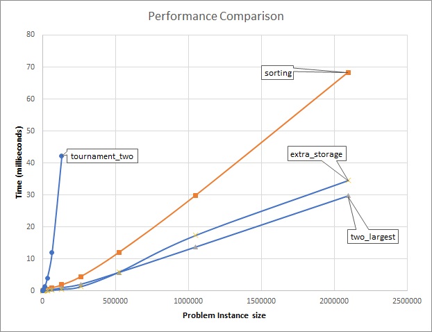
Figure 1-8. Runtime-performance comparison
While tournament_two is clever, it is significantly slower than the other
three alternatives. I can also claim that on large enough problem size
instances (in this case, 262,144 and larger) tournament_two is not a
reasonable algorithm to use, because there are algorithms that continue to
have acceptable performance even on large problem instances. Because the
graphed behavior of two_largest and extra_storage are so similar, they
appear to have more in common with each other than they do with sorting,
although I won’t be able to completely explain why until you read chapter
two. Now it’s time to explain the two useful fundamental concepts that
explain the inherent complexity of an algorithm.
Time Complexity and Space Complexity
It can be hard to count the number of elementary operations (such as
addition, variable assignment, control logic), because of the difference in
programming languages, plus the fact that some languages are executed by an
interpreter, such as Java and Python. But if you could count the total
number of operations executed by an algorithm, the goal of time
complexity is to come up with a function C(N) that counts the
number of elementary operations performed by an algorithm as a function of
N, the size of a problem instance.
Each elementary operation takes a fixed amount of time, t, based on the
CPU executing the operation. We model the time to perform the algorithm as
T(N) = t * C(N).
The following small example provides an insight that the structure of a
program is critical. For functions f0, f1, f2, and f3, you can
exactly compute how many times each one executes the operation ct = ct +
1 based on the input size, N. Table 1-5
contains the counts for a few values of N.
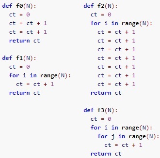
Figure 1-9. Four different functions with different performance profiles
The count for f0 is always the same, independent of N. The count for
f2 is always seven times greater than f1, and both of them double in
size as N doubles. In contrast, the count for f3 increases far more
rapidly; as you have seen before, as N doubles, the value of f3(N)
quadruples. Here, f1 and f2 are more similar to each other than they
are to f3. In the next chapter, we will explain the importance of for
loops, and nested for loops in evaluating an algorithm’s performance.
| N | f0 |
f1 |
f2 |
f3 |
|---|---|---|---|---|
512 |
|
|
|
|
1024 |
|
|
|
|
2048 |
|
|
|
|
When evaluating an algorithm, we also have to consider space complexity,
which accounts for extra memory required by an algorithm based on the size,
N, of a problem instance. Memory is a generic term for data stored in the
file system or the Random Access Memory (RAM) of a computer. two_largest
has minimal space requirements – three variables my_max, second, and
the iterator variable idx. No matter the size of the problem instance,
its extra space never changes. We say that this means the space complexity
is independent of the size of the problem instance, or constant. In
contrast, tournament_two constructs a tournament starting initially with
N/2 Match objects, ultimately constructing a total of N–1 of them. As N
increases, the total extra storage increases in a manner that is directly
proportional to the size of the problem instance. Building the tournament
structure is going to slow tournament_two down, when compared against
two_largest.
Still, there is one observation that holds. If you note in
Table 1-4, you can see that the timing results for columns
extra_storage and two_largest more-or-less double in subsequent rows.
This means that in both cases, the total time appears to be directly
proportional to the size of the problem instance which is doubling in
subsequent rows. This is an important observation, since these are both
more efficient than sorting which appears to follow a different, less
efficient trajectory. tournament_two is still the least efficient, with a
runtime performance that more than doubles, growing so rapidly that I don’t
bother executing it for large problem instances. In the next chapter, I
will present the mathematical tools necessary to analyze algorithm behavior
properly.
Note
The Tournament algorithm proposed here only works for an even number of values, N. How would you modify the algorithm to handle an odd number of N values?
Conclusion
This chapter provides an introduction to the rich and diverse field of algorithms. I showed how to model the performance of an algorithm on a problem instance of size N by counting the number of key operations it performs. You can also empirically evaluate the runtime performance of the implementation of an algorithm. In both cases, you can determine the order of growth of the algorithm as the problem instance size N doubles.
I introduced several key concepts, including:
-
Time Complexity as estimated by counting the number of key operations executed by an algorithm on a problem instance of size N
-
Space Complexity as estimated by the amount of memory required when an algorithm executes on a problem instance of size N
In the next chapter, I will introduce the mathematical tools of Asymptotic Analysis that will complete my explanation of the techniques needed to properly analyze algorithms.
Challenge Questions
-
Palindrome Word Detector: A palindrome word reads the same backward as forward, such as “madam”. Devise an algorithm that validates whether a word of N characters is a palindrome. Confirm empirically that it outperforms the following two alternatives:
defis_palindrome1(w):"""Create slice with negative step and confirm equality with w."""returnw[::-1]==wdefis_palindrome2(w):"""Strip outermost characters if same, return false when mismatch."""whilelen(w)>1:ifw[0]!=w[-1]:# if mismatch, return FalsereturnFalsew=w[1:-1]# strip characters on either end; repeatreturnTrue# must have been palindromeOnce you have this problem working, modify it to detect palindrome strings with spaces, punctuation, and mixed capitalization. For example, the following string should classify as a palindrome:
A man, a plan, a canal. Panama! -
Linear Time Median: A wonderful algorithm exists that efficiently locates the median value in an arbitrary list (for simplicity, assume list is odd size). Review the code (TBA) and count the number of times less-than is invoked. This implementation rearranges the arbitrary List as it processes.
A different implementation requires extra storage. Compare its performance with the one above.
-
Counting Sort: If you know that an arbitrary list,
A, only contains non-negative positive integers from 0 to M, then the following algorithm will properly sortAusing just an extra storage of size M.defcountingSort(A,M):counts=[0]*MforvinA:counts[v]+=1pos=0v=0whilepos<len(A):foridxinrange(counts[v]):A[pos+idx]=vpos+=counts[v]v+=1This code has nested loops - a for loop within a while loop. However, you can demonstrate that
A[pos+idx]=vonly executes N times.Conduct a performance analysis to demonstrate that the time to sort N integers in the range from
0to M doubles as the size of N doubles.You can eliminate the inner for loop, and improve the performance of this operation, using the ability in Python to replace a sublist using
sublist[left:right]=[2, 3, 4]. Make the change and empirically validate that it too doubles as N doubles, with over a 30% improvement in speed.