
Unsupervised Dictionary Optimization
Abstract
The core part of the learning-based local representation lies in the visual dictionary and its indexing structure, e.g., how to optimize the local feature-space quantization scheme. In Chapter 2, the design of the optimal interest-point detector was covered, while in this chapter, we introduce and discuss the way to optimize the dictionary construction-based on hierarchical metric learning unsupervised. We will show that the traditional Euclidean distance-based metric is unsuitable for k-means clustering, which would push clusterings located at dense regions and hence result in a biased distance metric. To deal with this issue, this chapter introduces density-based metric learning (DML) to refine the similarity metric in hierarchical clustering, which makes middle levels powerful and meaningful in retrieval. Based on an optimized VT model, we propose a novel idea to leverage the model hierarchy in a vertical boosting chain manner [84] to improve retrieval effectiveness. We will show that such an idea can generate a visual word distribution of the resulting dictionary to be more similar to the textual word distribution of documents. Furthermore, we also demonstrate that exploiting the VT hierarchy can improve its generativity across different databases. We propose a “VT shift” algorithm to transfer a vocabulary tree model into new databases, which efficiently maintains considerable performance without reclustering. Our proposed VT shift algorithm also enables incremental indexing of the vocabulary tree model for a changeable database in a scalable scenario. In this case our algorithm can efficiently include new data into model refinement without regenerating an entire model from the overall database.
3.1 Introduction
This chapter introduces density-based metric learning (DML) to refine the similarity metric in hierarchical clustering, which makes middle level words to be effective in retrieval. Based on an optimized VT model, we propose a novel idea to leverage the tree hierarchy in a vertical boosting chain manner [84] to improve retrieval effectiveness. Furthermore, we also demonstrate that exploiting the VT hierarchy can improve its generativity across different databases. We propose a “VT shift” algorithm to transfer a vocabulary tree model into new databases, which efficiently maintains considerable performance without reclustering. Our proposed VT shift algorithm also enables incremental indexing of the vocabulary tree for a changing database. In this case our algorithm can efficiently register new images into the database without regenerating an entire model from the overall database. For more detailed innovations of this chapter, please refer to our publication in IEEE International Conference on Computer Vision and Pattern Recognition 2009.
How Hierarchical Structure Affects VT-based Retrieval: Papers [31, 36] have shown that the k-means process would drift clusters to denser regions due to its “mean-shift”-like updating rule, which results in asymmetry division of feature space. We have found out that the hierarchical structure of VT would iteratively magnify such asymmetry division. More hierarchy levels result in more asymmetric similarity metrics in clustering. Therefore, the distribution of “visual words” would bias to denser regions in feature space (similar to random sampling), or even over-fit to feature density. However, to guarantee good “visual words” in hierarchical clustering, denser regions should correspond to more generic image patches, while sparser regions should be more discriminative. Recall that in TF-IDF the term weighting a visual word gains less weight when it appears in more images and vice versa. Hence, the hierarchical construction of VT would severely bias feature quantization: The discriminative patches (sparser regions that rarely appear in many images) would be coarsely quantized (i.e., give lower IDF and contribute less in ranking), while the general patches (denser regions that frequently appear in many images) would be finely quantized (i.e., gain inappropriately higher IDF in ranking). This is exactly the reason for inefficient IDF in [30] and [32]. In our consideration, the IDF inefficiency lies in the biased similarity metric, which is magnified by hierarchy clustering.
Another issue is that the nearest neighbor search within leaf nodes is inaccurate due to its local nature in the hierarchical tree structure, which would also degenerate matching accuracy. For validation, we compare the matching ratio of nearest neighbor search results both inside leaves and among overall feature space. For the vocabulary tree, the nearest neighbor search in leaf nodes is more inaccurate as the increase of nearest neighbor number in search scope. For validation, we compare the matching ratio of nearest neighbor (NN) search results both inside leaves and among overall feature space.
Table 3.1 presents the investigation of quantization errors in a 3-branch, 5-level vocabulary tree. We select 3K images from our urban street scene database to form the VT, with 0.5M features (average of 2K features in each visual word). We compare the matching ratio between global-scale NN and leaf-scale NN, in which global-scale is in the overall feature space while the leaf-scale is inside the leaf nodes.
Table 3.1
Hierarchical quantization errors measured using the overlapping rates (%)
| NN / GNP | 1 | 3 | 5 | 10 | 15 | 20 |
| 50 | 41.46% | 73.34% | 85.00% | 94.53% | 97.11% | 98.18% |
| 200 | 57.46% | 66.21% | 79.00% | 92.02% | 95.00% | 97.48% |
| 1,000 | 11.54% | 38.27% | 51.57% | 67.48% | 85.16% | 94.91% |
| 2,000 | 6.38% | 25.68% | 40.59% | 58.54% | 79.21% | 92.42% |
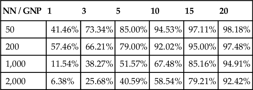
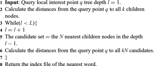
Greedy N-best Path
We extend the leaf-scale to include more local neighbors using greedy N-best path (GNP) [27]. The quantization error is evaluated by the matching ratio (%) to see to what extent the VT quantization would cause feature point mismatching (Figure 3.1). In Table 3.1, NN means the nearest neighbor search scope and GNP 1–5 means the numbers of branches we parallel in the GNP search extension. From Table 3.1 the match ratios between the inside-leaf and global-scale search results are extremely low when the GNP number is small. Algorithm 3.1 shows the detailed algorithm description.

Algorithm 3.1
Greedy N-best Path algorithm
Term Weighting Efficiency:
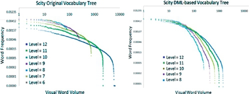
It is well-known that the Zipf’s Law1 describes the distribution of textual words in documents in which the most frequent words account for a large portion of word occurrences. Due to the inappropriate hierarchical tree division, the visual word distribution does not follow the Zipf’s Law (Figure 2.8).
Furthermore, with the increase in the hierarchical tree level, the word distribution becomes more and more uniform (Figure 3.1). Consequently, we can explain the phenomena observed in [32] that the IDF is less effective in large word volume. Subsequently, we can also infer that, in the current suboptimal hierarchical structure, the “stop words” removal technique won’t be very helpful since there are not very many visual words in images like “a” or “the” in documents. Our inference is validated by the “stop words” removal experiments in [32].
Dictionary Generality across Different Databases
When retrieving a new database, a common strategy is to recluster a VT model and regenerate all BoW vectors. However, in many cases the computational cost of hierarchical reclustering is a large burden in a large-scale scenario. Hence, it is natural to want to reuse the original VT model in a new database. However, it is very hard to construct a generalized vocabulary tree and a generalized visual codebook that are suitable for any scenario, especially when the new database has different data volumes (e.g., 1K images vs. 1M images) and different image properties (e.g., images taken by mobile phones vs. images taken by specialized cameras). If we directly represent a new database by an old VT model, the differences in feature volumes and distributions would cause hierarchical unbalance and mismatches in middle levels, resulting in over-fitted BoW vectors at the leaf level. On the other hand, to maintain a retrieval system that is effective in retrieval tasks, one important extension to improve system flexibility is to maintain the retrieval system in a scalable and incremental scenario. In such a case, the regeneration of the retrieval model and reindexing of image contents are over cost. It would be much more reasonable and effective to enable the retrieval model to be adaptive to data variance by model updating and incremental learning.
3.2 Density-Based Metric Learning
As shown above, the hierarchical structure will iteratively magnify the asymmetric quantization process in feature-space division, which resulted in suboptimal visual words and suboptimal IDF values in former papers [33] and [32]. To avoid this imbalance, we present a density-based metric learning (DML) algorithm: First, a density field is estimated in the original feature space (e.g., 128-dimensional SIFT space) to evaluate the distribution tightness of the local features. By extending denser clusters and shrinking sparser clusters, the similarity metric in k-means is modified to rectify the over-shorten or over-length quantization steps in hierarchical k-means. Subsequently, a refined VT is constructed by DML-based hierarchical k-means, which offers more “meaningful” tree nodes for retrieval.
3.2.1 Feature-Space Density-Field Estimation
To begin, we first introduce the definition of density field, which estimates the density of each SIFT point in the SIFT feature space as a discrete approximation. The density of a SIFT point in 128-dimensional SIFT feature space is defined by
where D(i) is the point density of the ith SIFT point, n is the total number of SIFT points in this dataset, and xj is the jth SIFT point. We adopt L2 distance to evaluate the distance between two SIFT points.
To make it efficient, we resort to estimating the density of each SIFT point using only its local neighbors as an approximation as follows:
where ![]() is the point density of the ith SIFT feature in its m neighborhood. We only need to calculate the local neighbors of SIFT by: (1) Cluster database features into k clusters: O(k * h * l), with h iterations to l points; and (2) nearest neighbor search in each cluster: O(l2/k). By a large k (e.g., 2000), our DML would be very efficient. Using a heap structure, it could be even faster.
is the point density of the ith SIFT feature in its m neighborhood. We only need to calculate the local neighbors of SIFT by: (1) Cluster database features into k clusters: O(k * h * l), with h iterations to l points; and (2) nearest neighbor search in each cluster: O(l2/k). By a large k (e.g., 2000), our DML would be very efficient. Using a heap structure, it could be even faster.
3.2.2 Learning a Metric for Quantization
From the above step, point-based density is estimated by neighborhood approximation. Subsequently, the similarity metric in hierarchical k-means are refined by density-based adaption as:
Similarity(c,i) is the similarity metric in DML-based k-means, which is the similarity between the cth cluster and the ith point; AveDen(c) is the average density of the SIFT points in the cth cluster; and Dis(ccenter,i) is the distance between the center SIFT point of cluster c and the ith SIFT point.
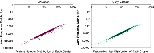
We explain this operation as follows: From the viewpoint of information theory, the generation of a “visual word” would cause information loss in the hierarchical quantization process. In particular, hierarchical k-means quantizes the sparser points with larger steps than the denser points. Therefore, the information loss is much more severe in the “probable informative” points (less likely to appear in most images) than the “probable uninformative” points (more likely to appear in most images). The proposed DML method decreases the overall quantization error by shortening the quantization steps for sparser regions to represent the “meaningful” points more precisely. Similar to textual words, the sparser regions in the SIFT feature space could be analogized to more meaningful textual words while the denser regions could be compared to less meaningful textual words, or even “stop words”. We demonstrate our inference by investigating the feature-word frequency in Figure 3.2. Our method can be also analogized to asymmetry quantization in signal processing.
To see how the DML-based method reduces the overall quantization error, we view the information loss of quantization using its weighted quantization error, in which the weight means the informative degree of the quantized word, which is evaluated by its IDF value. We denote the quantization error of the ith word as QA(i) (QA(i) > 0):
where ![]() is the kth feature dimension in the jth SIFT point of the ith cluster,
is the kth feature dimension in the jth SIFT point of the ith cluster, ![]() is the kth feature dimension of the ith cluster center, mi is the number of SIFT points in this cluster, and n is the number of words.
is the kth feature dimension of the ith cluster center, mi is the number of SIFT points in this cluster, and n is the number of words.
To evaluate the weighted quantization errors between the DML method and the original method, we compare their weighted signal-ratio rates as follows:
where wi is the IDF of the ith cluster as its word weight and px(x) and Δn(x) are the sampling probability and squared input-output difference of x, respectively. In its discrete case, Equation (3.5) can be replaced as Equation (3.6), in which we denote the DML case by superscript′ (such as n′, j″, and wi′):
The above equation can be further rewritten as follows:
The SIFT space is quantized into equal-numbered words, hence n = n′. Indeed, in Equation (3.8), ![]() is the quantization error in the ith cluster with mi points, identical to QA(i). Therefore, Equation (3.8) can be viewed as:
is the quantization error in the ith cluster with mi points, identical to QA(i). Therefore, Equation (3.8) can be viewed as:
Since denser regions appear in a larger portion of the images and hence would be assigned a very low IDF, it can be ignored in Equation (3.9), because its IDF is almost 0 due to the IDF’s log-like nature. On the contrary, in the sparser region, the quantization step is much more finite compared to the original method. Such a region has a much larger IDF and contributes more to the weighted quantization error. Based on Equation (3.8), QA(i) depends on: (1) point count mi and (2) distance between each point j and its word center. By DML construction, in sparser regions, both (1) and (2) are smaller than they were in the original k-means, which leads to smaller quantization error QA(i). In other words, our method quantizes “meaningful” regions with more finite steps, and “meaningless” regions with more coarse steps. Based on DML, we multiply the larger w with the smaller QA in Equation (3.9), while the larger QA corresponds to almost zero IDF weights. Evaluating the overall quantization error, it is straightforward that ![]() and SNRDML ≥ SNROrg. In other words, regardless of the quantization errors in meaningless words such as “a” and “the” (such words can be disregarded in similarity ranking as “stop words”), there are fewer weighted quantization errors in the DML-based tree.
and SNRDML ≥ SNROrg. In other words, regardless of the quantization errors in meaningless words such as “a” and “the” (such words can be disregarded in similarity ranking as “stop words”), there are fewer weighted quantization errors in the DML-based tree.
3.3 Chain-Structure Recognition
We further investigate how to better leverage such a model. We have found that the solutions for the (1) hierarchical quantization error and (2) unbalance feature division can be uniformly figured out by exploiting the DML-based tree hierarchy. This is because DML can address the unbalanced subspace division and the VT hierarchy itself contains the genesis of the quantization error.
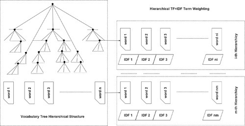
3.3.1 Chain Recognition in Dictionary Hierarchy
First, by expanding the TF-IDF term weighting procedure to hierarchical levels in the DML-based tree, the middle-level nodes are introduced into similarity ranking, which rectifies the magnified quantization errors in the leaves. In each hierarchical level, the IDF of the middle-node is calculated and recorded for middle-level matching. If the SIFT points are matched on a deeper level, their higher hierarchy would be hit by nature, meanwhile the ranking error of the leaf nodes caused by hierarchical quantization would be rectified in their higher hierarchy. Comparing to the GNP [27] method, our method offers an advantage in efficient computational cost, while maintaining comparable performance (see the subsequent Experimental section in this chapter).
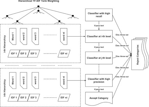
Secondly, we have discovered that the integration of visual words in VT hierarchy is a natural analogy to boosting chain classification [84, 102], which brings us to a new perspective on [16] how to leverage tree hierarchy. (In [16], middle levels are simply combined as a unified weighted BoW vector in similarity ranking, which is similar to adopted pyramid matching for high-dimensional input data as a Mercer kernel for image categorization.) In a hierarchical tree structure, by treating each level as a classifier, the upper level has higher recall, while the lower level has higher precision. This is straightforward because the higher level represents the abstract of category representation and is more uniform, in which the similarity comparison is coarser. On the contrary, in the finest level, the features are very limited and specified, leading to higher precision. In addition, the ranking results in each level being different due to their different quantization steps. Combining such hierarchical classifiers using a boosting chain manner can further improve retrieval.
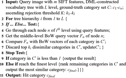
As presented in Figure 3.4, each level is treated as an “If...Else...” classifier that discards the least confident categories out of a vertical-ordered boosting chain for multi-evidence similarity ranking. In implementation, SIFT points belonging to the same query image are parallel, put in this hierarchical recognition chain, level by level, to incrementally reject most categories, as presented in Algorithm 3.2:
For each retrieved scene or object, the overwhelming majority of samples available are negative. Consequently it is natural to adopt simple classifiers to reject most of the negatives and then use complex classifiers to classify the promising samples. In our proposed algorithm, the vocabulary tree is considered as a hierarchical decision tree, based on which the cascade decision process is made at each hierarchy. A positive result past the higher level triggers the evaluation of the deeper level. Compared with a boosting chain that usually adopts boosting feature selection, our method utilizes each hierarchical level as a “visual word” feature for rejection due to its coarse-to-fine inherence.
3.4 Dictionary Transfer Learning
Facing an incremental database, when the recognition system receives new image batches, it is natural to retrain the recognition model all over again. Although good performance can be expected, the computational cost would be extremely unacceptable once the database volume is very large. In particular, to maintain our system for an online service, such cost would not be acceptable.
Algorithm 3.2
Vocabulary tree-based hierarchical recognition chain
The replacement of overall model retraining is that we only use a vocabulary tree to generate the BoW vectors for new images, without updating or retraining the VT-based recognition model. This is unrealistic, especially when there are new data patches coming.
Similar to the incremental case, we have discovered that the hierarchical tree structure can also facilitate the adaption of a VT-based retrieval model among different databases, which is important yet unexploited in literature. Different from reclustering the gigantic feature set of the new database, we present a novel tree adaption algorithm, VT shift, which enables: (1) adaption of the vocabulary tree among databases; and (2) incremental tree indexing in a dynamically updated database.
3.4.1 Cross-database Case
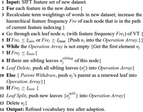
First, the SIFT features of the new database are sent through the original VT model, based on which the term weightings of the words are updated. The feature frequency of each leaf node reveals its rationality of existence and necessity of further expansion or removal. Leaf nodes that are either over-weighted or over-lightened would be adaptively re-assigned. Algorithm 3.2 presents our proposed VT shift algorithm.
Three operations are defined to iteratively refine the VT model to fit the new database:
1. Leaf Delete: If the feature frequency of a leaf is lower than a pre-defined minimum threshold, its features are reassigned back to its parent. Subsequently, this parent uses its sub-tree (with this parent as the root node) to assign the above features to their nearest leaves, except the deleted leaf.
2. Parent Withdrawal: If a leaf is the only child of its parent, and its feature frequency is lower than the minimum threshold, we withdraw this leaf and degrade its parent as a new leaf.
3. Leaf Split: If the feature frequency of a leaf is higher than the maximum threshold, we regrow this node into a sub-tree with the same branch factor in construction.
3.4.2 Incremental Transfer
We further leverage our proposed VT shift algorithm for incremental indexing in the SCity database. In our “Photo2Search” system-level implementation, we need a preliminary question about the genesis of new data. Algorithm 3.3 presents the details of the proposed VT Shift algorithm. Generally speaking, our system collects incremental scene images as well as their GPS locations from the three following sources:
1. Scene images uploaded by system administrators, which are directly sent into the database as a new data batch.
2. Query images sent by users to the server-end computer and images periodically crawled from Flickr API (we use both scene name and city name as crawling criterion), which are considered as Under Evaluated. For such data, pre-processing is conducted to further filter irrelevance: We treat each new image as a query example, for scene retrieval, if the cosine distance between this query and the best matched image is lower than Tmax (i.e., they are similar enough), we add this image into the new data batch in our database.
To provide consistent service along with the process of incremental indexing, our system maintains two central computers on the server side. Each maintains a location recognition system that is set to be identical after finishing one round of adaption. Initially, the status of one system is set as active while the other as inactive. Active means this server program is now utilized to provide service; inactive means this server program is now utilized for incremental indexing. Once the inactive program receives a new batch of scene images, we first investigate whether it is necessary to activate the incremental indexing process. If so, we conduct incremental indexing and switch its inactive status to active, and vice versa; otherwise, these images are temporarily stored and added into subsequent new image batches.
Facing a new image batch, it is not always necessary to activate the incremental indexing process in the inactive server. If the distribution of the new data is almost identical to that of the original dataset, adaption could be postponed for the subsequent images. Hence, to reduce the computational cost in large data corpora, we conduct model adaption once either of following cases is true: (1) the volume of the new images is large enough or (2) the distribution of the new images is extremely diverse from that of the original database. We present an adaption trigger criterion using Kullback-Leibler (KL) diversity-based relative entropy estimation as in Figure 3.3 and explained in detail as follows.
Algorithm 3.3
Dictionary transfer algorithm: VT Shift

First, data distribution is measured by its sample density, which is identical to the density field in DML-based tree construction. Facing a new data batch, we evaluate the data dissimilarity DiverAccu between the original database and the new data batch by their density-based KL-like relative entropy estimation:
in which ![]() is the density of the new data at the ith data point in the mth neighborhood; Dorg(Nearest(i),m) is the density of the old data at the nearest old point of the ith new data in the mth neighborhood. It can be observed from the above equation that data diversity increases as: (1) the volume of the new data batch increases; (2) the distribution of the original database and new data batch are more diverse. Consequently, we control the incremental indexing process by trigger criterion as follows: When fusing a new data batch into the original database, the point density in the original database need not be updated. Indeed, their former density estimations can be partially preserved and only need to be modified by new data (Algorithm 3.4):
is the density of the new data at the ith data point in the mth neighborhood; Dorg(Nearest(i),m) is the density of the old data at the nearest old point of the ith new data in the mth neighborhood. It can be observed from the above equation that data diversity increases as: (1) the volume of the new data batch increases; (2) the distribution of the original database and new data batch are more diverse. Consequently, we control the incremental indexing process by trigger criterion as follows: When fusing a new data batch into the original database, the point density in the original database need not be updated. Indeed, their former density estimations can be partially preserved and only need to be modified by new data (Algorithm 3.4):
where k is the number of remaining original points in m nearest neighbors, which is achieved by comparing the new data with the former-stored m nearest neighbors of each point.
Algorithm 3.4
Visual dictionary transfer learning trigger detection
3.5 Experiments
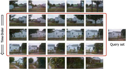
In our experiments, two databases are investigated: Scity and UKBench. Scity consists of 20K street-side photos, captured along Seattle urban streets by a car automatically, as shown in Figures 3.5 and 3.6. We resized these photos to 400 × 300 pixels and extracted 300 features from each photo on average. Every six successive photos are grouped as a scene. The UKBench database contains 10K images with 2.5K objects (four images per category). We also leverage UKBench for performance evaluation, but not for scene recognition task. In both databases, each category is divided into both a query set (test performance) and a ground truth set (create VT): In the Scity database, the last image of each scene is utilized for a query test while the former five images are adopted to construct the ground truth set. In the UKBench database (2.5K categories), the one image from each category is adopted to construct the query set while the rest are used to construct the ground truth set.
We use Success Rate at N (SR@N) to evaluate system performance. This measurement is commonly used in evaluating Question Answering (QA) systems. SR@N represents the probability of finding a correct answer within the top N results. Given n queries, SR@N is defined as Equation (3.1), in which ![]() is the jth correct answer of the qth query,
is the jth correct answer of the qth query, ![]() is its position, and Θ() is the Heaviside function: Θ(x) = 1, if x ≥ 0, and Θ(x) = 0, otherwise.
is its position, and Θ() is the Heaviside function: Θ(x) = 1, if x ≥ 0, and Θ(x) = 0, otherwise.

We build a 2-branch, 12-level vocabulary tree for both Scity and UKBench. The reason we leverage 2 divisions at each level is because of the consideration of large-scale application in real-world systems. With the same dictionary size, the search speed is with the log nature of branch number. For a VT with fixed word size (m), the search cost comparison of a-branch VT and b-branch VT for one SIFT point is ![]() , which means the smaller branch factor results in much faster search speed. In both trees, if a node has less than 2,000 features, we stop its k-mean division, no matter whether it achieves the deepest level or not. In tree adaption, the maximum threshold ξmax is set as 20,000; the minimum threshold ξmin is set as 500.
, which means the smaller branch factor results in much faster search speed. In both trees, if a node has less than 2,000 features, we stop its k-mean division, no matter whether it achieves the deepest level or not. In tree adaption, the maximum threshold ξmax is set as 20,000; the minimum threshold ξmin is set as 500.
3.5.1 Quantitative results
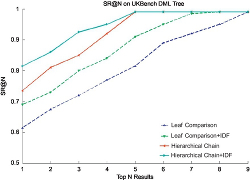
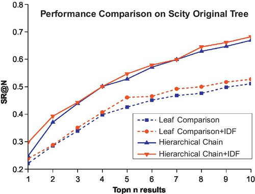
Figure 3.7 presents the SR@N in UKBench before and after DML, both of which conduct three comparisons: (1) leaf comparison, in which only leaf nodes are used in similarity ranking; (2) hierarchical chain, in which we adopt the hierarchical recognition chain for multi-evidence recognition; and (3) hierarchical chain + IDF, in which each level of the hierarchical recognition chain is combined with the IDF weights of their nodes in similarity ranking.
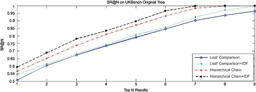
It is obvious that before DML learning, the real powers of the hierarchical recognition chain as well as the hierarchical IDF cannot be revealed well. But combinational performance enhancements of both methods after DML learning are significant, almost 20% over leaf-level baseline. Comparing Figure 3.7 with Figure 3.8, it is easy to see that the DML-based tree performs fairly better than the original tree, almost 20% enhancement to the best results. The same result holds in Scity as shown in Figures 3.9–3.10.
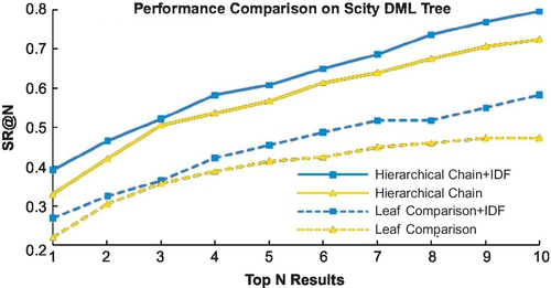
Indeed, this phenomenon can be expressed by Figure 3.11, after DML-based construction: the word distribution in the hierarchical level would follow Zipf’s Law better, which means not only middle-level nodes but also their IDF would be more discriminative and more meaningful.
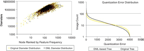
Actually, without DML-based optimization, the hierarchical k-means would be biased to the denser regions and incorrectly divide them deeper and tighter rather than the sparse regions. This bias is hierarchically accumulated and wrongly assigns such regions with high IDF in recognition. This is why the use of IDF is not better in the original tree [30, 32], while it is better in the DML-based tree. Figure 3.12 further explains this enhancement in UKBench. On the left, the cluster diameter distribution in the 12th level is ranked by feature frequency. By DML construction, the diameter distribution is more uniform, so feature-space division is more uniform; on the right, quantization error distribution is ranked by image counts of clusters. The quantization errors with more images are higher, but in clusters with fewer images they are much lower. An intuitive motivation of DML-based tree construction is to refine the original distance metric in k-means clustering, which is achieved by generating more clusters in denser regions and less clusters in sparser regions. Since VT hierarchy magnifies unbalanced space division, DML revises such bias to rectify such unbalance.
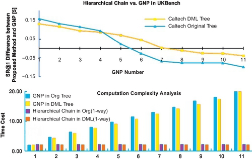
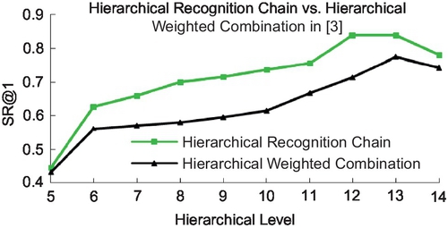
We further investigate the efficiency of the hierarchical recognition chain. Figure 3.13 presents a comparison between our method and GNP [27]. We also evaluate how the chain level affects the recognition performance in UKBench. The method from Nister [16] that combines middle levels into a unified BoW vector is also given (Fig. 3.14). Compared to [16], the proposed method can achieve better performance. When n > 14, performance begins to degenerate due to over-quantization. Compared to [16], VT has an advantage in efficient search in the large-scale case. Its cost is accuracy degeneration compared to solely SIFT matching. On the contrary, AKM in [10] merits in matching precision but it’s time-consuming: (1) It use float k-means; and (2) to ensure precision, the k-d forest is also slow.
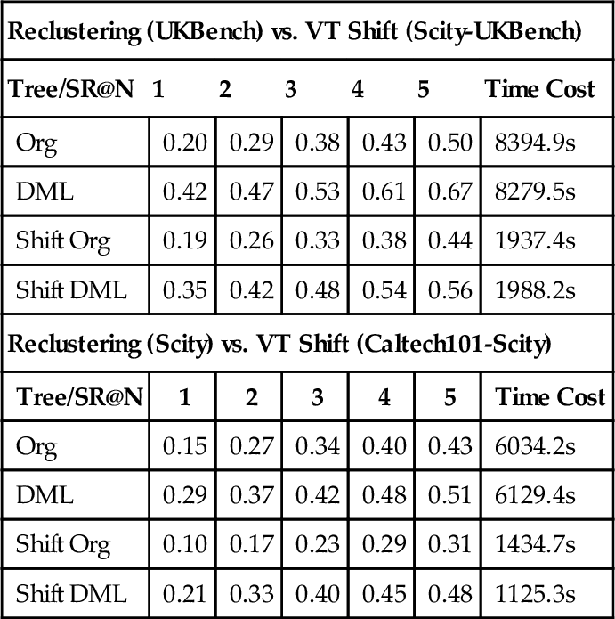
We evaluate our proposed VT shift algorithm with the following experiments: Figures 3.15–3.16 present the VT shift performance between UKBench and Scity with different volumes (9K vs. 20K) and applications (scene vs. object). It is obvious that direct application of the dictionary across databases with different constitutions would cause severe performance degradation (Figure 3.17). However, the VT shift algorithm can well address the tree adaption problem. Table 3.2 presents the advantage of the DML-based tree in VT Shift operation over the original tree in both databases.
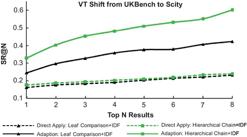
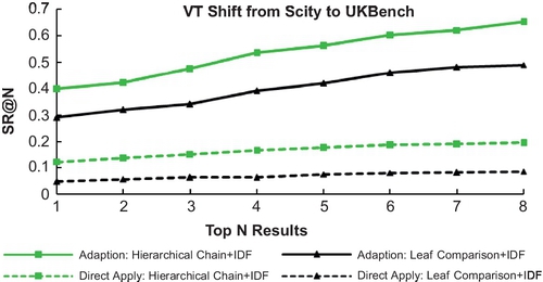
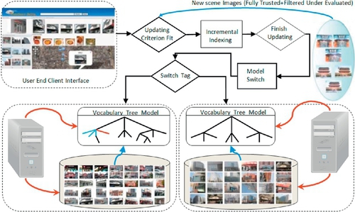
Table 3.2
Performance analysis of VT Shift
| Reclustering (UKBench) vs. VT Shift (Scity-UKBench) | ||||||
| Tree/SR@N | 1 | 2 | 3 | 4 | 5 | Time Cost |
| Org | 0.20 | 0.29 | 0.38 | 0.43 | 0.50 | 8394.9s |
| DML | 0.42 | 0.47 | 0.53 | 0.61 | 0.67 | 8279.5s |
| Shift Org | 0.19 | 0.26 | 0.33 | 0.38 | 0.44 | 1937.4s |
| Shift DML | 0.35 | 0.42 | 0.48 | 0.54 | 0.56 | 1988.2s |
| Reclustering (Scity) vs. VT Shift (Caltech101-Scity) | ||||||
| Tree/SR@N | 1 | 2 | 3 | 4 | 5 | Time Cost |
| Org | 0.15 | 0.27 | 0.34 | 0.40 | 0.43 | 6034.2s |
| DML | 0.29 | 0.37 | 0.42 | 0.48 | 0.51 | 6129.4s |
| Shift Org | 0.10 | 0.17 | 0.23 | 0.29 | 0.31 | 1434.7s |
| Shift DML | 0.21 | 0.33 | 0.40 | 0.45 | 0.48 | 1125.3s |
We further leverage our proposed VT shift algorithm for incremental indexing in the SCity database. In our “Photo2Search” system-level implementation, we should figure out a preliminary question about the genesis of new data (Figure 3.18). Generally speaking, our system collects incremental scene images as well as their GPS locations from the two following sources:
1. Scene images uploaded by system administrators, which are directly sent to the database as a new data batch.
2. Query images sent by users to the server-end computer and images periodically crawled from the Flickr API (we use both scene name and city name as crawling criterion), which are considered as under evaluated. For such data, pre-processing is conducted to further filter irrelevance: We treat each new image as a query example, for scene retrieval; if the cosine distance between this query and the best matched image is lower than Tmax (i.e., they are similar enough), we add this image into a new data batch in our database.
To provide consistent service along with the process of incremental indexing, our system maintains two central computers on the server side. Each maintains a location recognition system that is set to be identical after finishing one round of adaption. Initially, the status of one system is set as active while the other as inactive. Active means this server program is now utilized to provide service; inactive means this server program is now utilized for incremental indexing. Once the inactive program receives a new batch of scene images, we first investigate whether it is necessary to activate the incremental indexing process. If so, we conduct incremental indexing and switch its inactive status to active and vice versa; otherwise, these images are temporally stored and added into consequent new image batches.
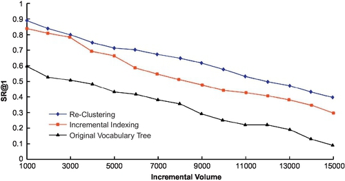
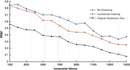
Figure 3.19 presents the performance comparison between our proposed method and methods (1) and (2). With the increase of database volume, the SR@1 performance is naturally decreased. Although reclustering performs better than our proposed method, its time cost is unacceptable compared to both incremental indexing and simply using original VT to generate new BoW vectors. Our method can maintain comparable performance (less than 10% degradation than comparing to reclustering), while requiring fairly limited computational cost (24% cost compared to reclustering).
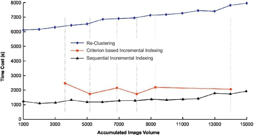
We compare our proposed incremental indexing with method 1), reclustering of an entire renewed database (it has the best performance as the performance upper limit and 2), original VT that only regenerates BoW vectors for new images. It has no adaption in tree structure and is the performance baseline. We not only compare their recognition performance using SR@1 (Figure 3.18) but also compare their adaption computation cost using their computational costs in Figure 3.20.
3.6 Summary
This chapter demonstrated that exploiting the hierarchical structure of a vocabulary tree can largely benefit patch-based visual retrieval. We discovered that the hierarchical VT structure can allow us to (1) optimize visual dictionary generation; (2) reduce quantization errors in BoW representation; and (3) transfer the patch-based retrieval model across different databases. We presented a density-based metric learning (DML) algorithm to unsupervised optimize tree construction, which reduces both unbalanced feature division and quantization error. Subsequently, we introduced a hierarchical recognition chain to exploit middle levels to improve retrieval performance, which has an advantage in algorithm efficiency compared to GNP [5]. Compared to the–current retrieval baselines, our overall performance enhancement is 6–10% in the UKBench database and over 10-20% in the Scity scene database. Finally, we also discovered that the hierarchical tree structure can make the VT model reapplicable across different databases as well as adaptive to database variation to maintain considerable performance without reclustering. In our future work we will further investigate the influences of visual word synonymous and multivocal to improve retrieval efficiency.