
6 Transportation (Medium- and High-Speed) SLIM Design
6.1 Introduction
We define transportation as urban and interurban public people or freight movers with vehicle suspension on wheels or via MAGLEVs.
The main difference between magnetic and wheel suspension of people movers from the SLIM design point of view is the treatment of net normal force Fn.
As shown in Chapter 3, Fn is reasonably low (three times rated propulsion force in aluminum-on-iron SLIMs) if the efficiency is the main target of the design. Fn switches from repulsion to attraction force as the slip (secondary) frequency decreases; the switching point condition, however, corresponds to a rather large slip frequency (Chapter 3), which may not be acceptable as it produces high losses (lower efficiency) in the SLIM.
It is thus advisable for SLIM-MAGLEVs to arrange the secondary track above the SLIM, on the two sides of the vehicle, and to use the attraction normal force of SLIMs at lower slip frequency, that is, better efficiency.
To complement the main (SLIM) magnetic suspension system, actively controlled dc electromagnets with (or without) PMs are placed also on board (Figure 6.1a). For vehicles on wheels, the net attraction normal force may be limited to a certain value that does not produce excessive noise and vibration at vehicle start while it enhances a little the mechanical adhesion of wheels (Figure 6.1b). Also for some SLIM-MAGLEVs, the SLIM is still placed above the track, and thus, the net normal force of LIM has to be counteracted by the dc-controlled electromagnets that provide vehicle levitation (Figure 6.1c); the SLIM slip frequency may also be controlled to have the net normal force close to zero, but that may compromise efficiency too much.
The previous chapter has dealt with the design of tubular-secondary SLIMs, while in this chapter, only the SLIM with aluminum-on-iron secondary will be treated, as it seems the practical way to follow for a reasonable passive track cost for long travels, as in transportation (even for industrial transport, over a few tens of meters).
Again, the electromagnetic design aspects will be the main target, but at least for urban SLIM vehicles, some issues of secondary losses and temperature around stop stations will be approached in some detail.
Case studies will accompany the design methodologies, for urban SLIM vehicles (max speed >34 m/s) and for interurban vehicles (100 m/s).
6.2 Urban Slim Vehicles (Medium Speeds)
The design methodology by a numerical example includes (1) the specifications; (2) additional data; (3) main dimensions, parameters, and performance; (4) secondary thermal design issues and performance numerical results.
Specifications
Peak thrust up to base speed (ub = 12 m/s): 12 kN
Thrust at max speed (ubmax=34 m/s): 3 kN
Starting current 500–600 A
Supply: DC supply at 700 Vdc and PWM voltage-source IGBT inverter on vehicle (max voltage/phase (RMS): 300 V)
Aluminum-on-iron secondary track
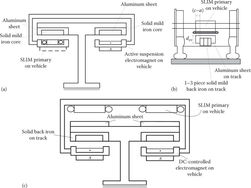
FIGURE 6.1 SLIM arrangements for transportation: (a) for MAGLEVs, (b) for vehicles on wheels, (c) alternative MAGLEV.
Additional data from prior experience
As even with three-piece secondary solid mild back iron, the field penetration depth, under heavy saturation, is not going to reach more than 15–20 mm, the pole pitch has to be limited to perhaps 0.22–0.27 m; a three-piece solid back-iron secondary is chosen here.
The tight curves to be handled in urban transportation restrict the primary on-board length to 2–3 m.
To reduce end-coil length, the primary winding should have two layers and chorded coils, which leads to two-layer windings with 2p + 1 poles and half-filled end-pole slots.
The number of poles for urban SLIM vehicles is thus limited to 7, 9, and 11; the lower limit is imposed by the necessity to limit the dynamic (and static) end effect.
The airgap flux density at maximum (peak) thrust has to be limited due to limited secondary back-iron skin effect, but also to limit the net normal force, with its consequences, as discussed earlier. Values of B1gmax = 0.20 – 0.35 T are considered feasible.
The optimum equivalent goodness factor Geo (Chapter 3) is considered here the key design variable; with these restrictions, for 2p + 1 = 11 and τ = 0.255 m, from Chapter 3 (Geo)2p=10 = 24; the equivalent goodness factor varies with respect to slip frequency, current (due to magnetic saturation), and with the airgap variation due to track irregularities, so Geo value has to be observed at rated slip (and peak speed).
The dynamic end effect may not be neglected even for this urban application, though the optimum goodness factor strikes a good compromise between thrust/weight and ηn cos φn (which, in turn, is related to energy usage rate and inverter initial costs).
In presence of dynamic end effects, it seems more practical to design (size) the SLIM rather in the 1D technical field theory (Chapter 3) than in equivalent circuit terms; the end effect correction coefficient Ke(Ge, p, s), inserted in the circuit model, may be added at the end to the other circuit parameters; their dependence on current and slip frequency makes them less useful in assessing quickly the performance, unless convenient curve-fitting approximations of their variations are not produced.
The mechanical airgap g = 8–10 mm for urban SLIM vehicles (with safety devices to secure it), for handling realistic track irregularities.
Aluminum and back-iron pieces are added together to make the track; they produce some speed-tied frequency pulsations in the thrust and normal force, with only 2%–3% average thrust reduction for secondary sections in the 1–2 m length range; bolt joints may be added, but they are too costly for a small beneficial effect [1].
The thickness of aluminum sheet is dAl=4−6 mm, as a compromise between track costs and SLIM performance and costs; a large thickness leads to better goodness factor for given mechanical gap. But at the price of higher magnetization current (lower power factor), dAl may become a variable to optimize, for a given application, when a multiple-target objective function is used.
The primary stack width 2a = 0.2−0.3 mm, again to limit the secondary track costs; as 2a/τ ≈ ∼0.8−1.2, the edge effect is also limited this way; finally, the aluminum sheet overhang cross section should be τdAl/π. The depth of the aluminum overhang when placed adjacent to secondary back iron dov < 3dAl, to limit the skin effect in this zone also, so (c − a)e = τdAl/dov > τ/12, while for “pure” aluminum sheet, (c − a) > τ/π.
This additional data have to be corroborated with the specifications, by adjusting the number of poles 2p + 1, pole pitch, and stack width, to secure a specific thrust in the range of 2 N/cm2 for the case in point.
The secondary back-iron width wi ≈ 2a + 0.02 m.
The rated slip (once the optimum goodness factor is chosen for rated thrust as a compromise between conventional and with-end-effect-considered performance and primary weight) is chosen not very far away from the condition SrGeo = 1, which corresponds to max conventional thrust/mmf. For urban SLIM vehicles, we may choose SrGeo ≈ 2 for max speed Umax = 34 m/s corresponding thrust Fxn = 3 kN.
For the peak thrust at standstill and then up to base speed (Ub = 12 m/s), the same conditions may be kept; that is, constant slip (secondary) frequency f2 =f2r = S · f1max; the primary frequency f1max corresponds to max speed (here, Umax = 34 m/s).
If, as the required thrust decreases, the slip frequency is increased, the conventional losses increase, but the average end effect also diminishes (slip increases); a slight increase in f2 with speed becomes thus practical; care must be exercised, as f2 influences notably the total normal force also.
Main dimensions
First, let us choose from paragraph (2) a few notable SLIM sizing data
Aluminum sheet thickness dAl=6 mm (initial value)
Airgap g = 8 mm
Pole pitch τ = 0.25 m (initial value)
Slip frequency (constant) f2r=6 Hz, at base speed
Stack width 2a = 0.27 m
The aluminum equivalent overhang (c − a) = τ/π c − a = τ/π
2p + 1 = 11 poles two-layer primary winding with half-filled end-pole slots
The design start is related to the optimum goodness factor
where σe is the equivalent aluminum conductivity including skin effect at rated slip frequency, edge effect, and solid (3 laminations) back-iron thrust and loss contribution: ge ≈ (g + dAl)*KcKFg
Assuming f2r = 8 Hz at max speed, with τ = 0.25 m and Umax = 34 m/s, the maximum frequency f1max becomes
From (6.1) to (6.2), the ratio σe/(1 + Kss) may be found:
Let us remember that the aluminum electrical conductivity is σAl ≈ 3.25 × 10⁷ (Ω m)−1. This shows that the aluminum edge effect and the solid back-iron contribution to σe have to be substantial (or the pole pitch may simply be decreased, even below Geo=24). Let us consider first an approximate value of aluminum edge effect Ktr on its electrical conductivity (though the more involved expression derived in Chapter 3 may be used in a design computer code):
So the iron contribution to secondary conductivity Kiσ (3.46) and the airgap through Kss (3.44) should amount to
But
From (3.42) for iron field penetration depth δiron (3.15), Ktri is
(i = 3 “laminations” in the secondary back iron)
The secondary back-iron permeability may only approximately be calculated as in (3.17):
with Bg1 the airgap flux density at max speed and corresponding thrust (3 kN). Considering Bg1max = 0.3 T at max thrust (12 kN, to limit the normal force), it follows that for thrust proportional to current squared and flux density proportional to current Bg1 ≈ Bg1max/2 = 0.15 T; considering end effect, we may use Bg1 = 0.22 T.
For Btmax = 2.2 T and Hm = 50,000 A/m for mild solid steel of secondary, μiron (on its surface) is
so
The depth of penetration looks large, but let us remember that at same f2r=8 Hz, the maximum flux density has to be flown at start and up to base speed (for Fxmax = 12 kN). So condition (6.9) has to be satisfied rather for Bg1max = 0.3 T:
The factor Kss = 1.5 in (6.9) takes care of back-iron field redistribution with doubled flux density, due to primary limited length (Chapter 3).
However, it seems clear that even an δi ≈ 25 mm would suffice, which may be obtained with an iron surface flux density of around 2.0 T and Hm = 30,000 A/m.
Additionally, two-lamination back iron may be used, for which Kiron ≈ 4, μiron ≈ 53μ0, and δ1 ≈ 25 mm. Consequently from (6.6),
So, returning to (6.5),
The difference between the required and obtained ratio is acceptably small, and thus, the 25 mm thick solid back iron of secondary made of two-lamination (pieces) stands. But it has to be noticed that the iron contribution (to thrust, losses, and magnetization current) depends heavily on primary current (via magnetic saturation) for given slip frequency; a robust thrust control loop is required as also the airgap may vary due to track irregularities, etc.
For simplicity, the optimum goodness factor at Bg1max = 0.22 T and f2r = 8 Hz, Geo = 24 will be considered further on in the design, though above base speed (ub=12 m/s) up to ubmax=34 m/s, the thrust decreases and so does the current, but less than proportional, because of smaller penetration depth of iron and thus a larger demand on magnetization current. Also, the goodness factor decreases somewhat below Geo=24. In a rather complete design, such conflicting influences should be accounted for.
One more aspect is related to the occurrence of a leakage inductance effect of iron eddy currents in the secondary back iron, because the skin effect inflicts eddy current density phase shifting, besides magnitude reduction, along the back-iron depth. At 50 Hz, it has been proved that ωlL′2n ≈ R′2l of iron; at 8 Hz, the influence is notably smaller, and so is the iron influence on losses (and thrust), so a first approximation L′2li ≈ 0. Also the airgap fringing coefficient Kfg accounts approximately for the skin effect leakage inductance in aluminum, which, again, is rather small.
4. Peak thrust capability
To continue the design, the peak thrust capability required below base speed is checked in terms of primary slotting and winding loss suitability for 2p + 1 = 11 poles, τ = 0.25 m, and 2a = 0.27 m for 12 kN thrust.
First, let us calculate the peak specific thrust fxspeak:
This is a reasonable value, to expect good efficiency, especially at lower values of thrust required above base speed.
It is not sure that the LIM will provide at, f1 =f2r=6 Hz at start, the peak thrust at reasonable losses with the main geometry already in place. For 6 Hz, the goodness factor at start will be
This value is far away from the maximum thrust/current at start where Geso = 1. Though reducing further f2 < 6 Hz at start would lead to vibration and noise in wheeled vehicles, the higher normal force in MAGLEVs may be advantageously used at start to assist the dc-controlled electromagnets in magnetic suspension.
The flux density Bg1max = 0.3 T is (5.24)
With τ = 0.25 m, slot openings as wide as bs1 = 18 mm are allowed (bs1/(g + dAl) = 18/14 < 2/1!), without heavy influence of Carter coefficient on airgap flux-density space harmonics augmentation (Figure 6.2).
So q1 = 3 slots/pole/phase, γ/τ=7/9 (chorded coils) with slot pitching, τs1 = τ/q1m1 = 0.25/9 = 0.027 m=27.77 mm, and bs1 = 18 mm; the primary tooth width bt1 = τs1 − bs1 = 27.77 − 18 = 9.77 mm (with up to 0.3 T in the airgap, no stator teeth heavy saturation may occur).
From (6.19), the peak phase Ampere turns, w1I1peak (RMS value), is
The number of coils/phase corresponds to 10 (not 11) poles, but fully filled (two layers) and thus the peak Ampere turn per slot 2ncI1peak is
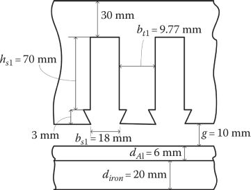
FIGURE 6.2 Longitudinal geometry of designed SLIM for urban transportation.
This mmf has to be sustained for Bgmax = 0.3 T and f20 = 6 Hz up to base speed. It is not yet sure that it will provide the required thrust. But before that, let us see if reasonable slot geometry is feasible.
For a bs1 = 18 mm wide and hs1 = 70 mm deep slot, with a slot filling factor Kfill=0.55, the current density jcop for peak thrust would be (Figure 6.2)
The peak thrust check for this peak Ampere turns/phase value is now done, at standstill (4.11):
where Lm is the magnetization inductance (5.6):
From (6.23),
So a smaller flux density than 0.3 T in the airgap is necessary to produce the peak thrust. Consequently w1I1peak has to be reduced approximately by the square root of thrust overestimation:
So the peak current density in (6.22) becomes jcopt=6.59 × 48,665/68,050=4.712 A/mm2. This is quite a reasonable value, which may be sustained during acceleration cycles from zero to base speed. Also Bg1max ≈ 0.215 T, and thus, the secondary back-iron depth may be reduced to 20 mm.
Let us consider w1 = 90 turns/phase, to yield a peak phase current I1peak=(w1I1peak)/ w1=48,665/90 = 540 A < 600 A (see the specifications).
With w1 = 90 turns/phase and 30 coils/phase in series, it follows that a coil has only three turns, which means that twisted-cable turns should be used in preformed coils. The nonuniform flux-density distribution along primary length due to dynamic end effects above base speed precludes in general the usage of multiple current paths in parallel.
5. Dynamic end effect influence
Dynamic end effect influence manifests itself on thrust, secondary and primary winding losses, and, to a smaller degree, on power factor.
The key influence, as described in Chapters 3 and 4, is the ratio fe = Fxe/Fxc, with Fxe—end effect force and Fxc—conventional thrust (without end effect).
From (3.70),
Alternatively Ref. [2] has introduced the emf coefficient Ke=E1e/E1c, where E1e is the end effect emf and E1c is the conventional emf (without end effect), as followed in Chapter 4 (4.37).
So the total thrust Fx is
as the total emf per phase E1 is
As evident, both fe and Ke depend at least on speed and slip (or on goodness factor, which includes primary frequency and slip) for given SLIM geometry.
Only in the low slip region (as described in Chapter 3) coefficient fe varies monotonously with slip and increases rather monotonously with speed.
The slip used, in the present case study, at maximum speed (34 m/s) corresponds to 6–8 Hz in the secondary and 74(76) Hz in the primary.
Considering constant influences of edge and skin effects fe, (6.27) may be straightforwardly calculated as a function of speed (frequency f1, that is Ge) for given slip S, and then its dependence on speed is evident u=2τ(f1 − f2).
For the case in point, and similar ones [3], a rather linear dependence of fe with f1 (speed) is obtained.
When designing the SLIM at optimum goodness factor for a slip S ≈ 0.1, the end effect influence on thrust (Fe), which depends on the goodness factor Ge and on the number of poles (the speed is implicit in Ge), for 2p = 10, calculated from (6.27), amounts in general to maximum 20%.
Similarly from (3.74) to (3.75), the secondary aluminum iron eddy current losses p2 and the airgap reactive power Q2 are calculated.
By the balance of powers, input active power P1 and reactive power Q2, efficiency ηn, and power factor cos φ1 are as follows:
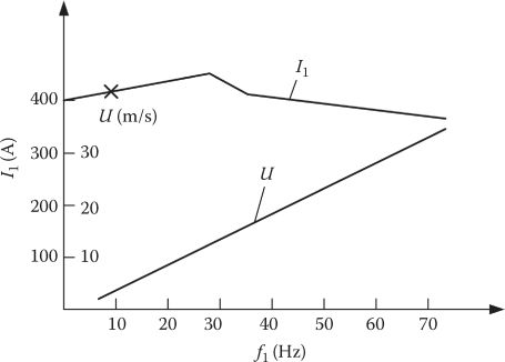
FIGURE 6.3 Imposed current and speed versus primary frequency.
This way, with a limited effort, the main SLIM performance for given I1, s, Ge(f1) is obtained, including all main influences of dynamic end effect (on thrust, losses, and power factor).
Finally, the modified equivalent circuit to account for dynamic end effects (Figure 4.14) may be explicit and curve fitted, if so needed for further simplification.
For control purposes, the factor Ke (dependent on speed, slip, current) alone may be used in the space phasor model (4.74) to account for dynamic end effects.
Note: As the secondary back-iron saturation has a heavy influence on equivalent goodness factor, at high speed, the end effect influence changes notably, and thus, a robust thrust (or at least speed) control is required.
To save space with tedious, but, as seen earlier, rather straightforward mathematical developments, Figures 6.3 through 6.5 present final results on performance of SLIM with data very close to ones in our case study, but with an aluminum sheet of only 4 mm thickness, where dynamic end effect influence was considered by a coefficient fe (or Ke), which is only 0.15 at max speed and S=0.1 and varies linearly with speed, for f2 = 8 Hz [3].
The results in Figures 6.4 through 6.5 warrant remarks such as the following:
A rather good efficiency is obtained (around 0.8) but the power factor is only around 0.5, which imposes notable oversizing of the inverter.
The normal force is in general about three times larger than thrust, which should be acceptable, especially in a wheeled vehicle.
A sizeable amount of power is retrieved during regenerative breaking, and the dc power bus should be able to handle it (to transfer it back to the ac power system or to the other vehicles).
6. Secondary thermal design
The thermal design of SLIM primary is similar to that of rotary IMs, with only a few peculiarities, such as the fact that it is placed in the way of the ambient air (below the vehicle) at vehicle speed and the heat transfer from secondary to primary (and vice versa) may be neglected due to the large mechanical airgap. As the thrust at low speed is high (peak thrust), this situation has to be considered when designing the cooling system for SLIM primary.
The secondary cooling raises special problems, especially around stop stations when the frequency of vehicle passage at low speed is large.
It may be practical to calculate the minimum head (lead) time between two successive vehicles that start from the same secondary section such that the maximum temperature of the latter does not surpass 120°–150° in general.
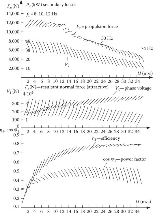
FIGURE 6.4 Thrust Fx, secondary losses p2, normal force Fn, phase voltage V1, efficiency η1, and power factor cosφ1 versus speed for urban SLIM.
The secondary temperature influences the goodness factor, and thus, the thrust and secondary losses produced at standstill vary and should be accounted for by a verification of the worst scenario startup conditions (maximum temperature of secondary).
Let us consider peak thrust Fxp with vehicle mass M; the acceleration ams is
The thermal energy, Wp, in 1 m length of secondary, while a vehicle passes over it, is
where
n is the number of successive motors on a vehicle
L is the length of the primary (L ≈ (2p + 1)τ)
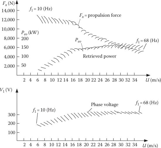
FIGURE 6.5 Regenerative braking: thrust Fx, retrieved power p2, and phase voltage.
But the secondary losses at start are simply
(p2)S=1 is in fact the worst situation because the vehicle moves from the secondary section of start quite rapidly.
With T as the minimum interval between two successive vehicles and m vehicles present over the same section since their start in the morning (when secondary temperature was equal to the ambient temperature), the secondary temperature θ(t) becomes
When the temperature stabilizes,
And thus
From (6.34) through (6.37), it follows that
with
Cs as the equivalent specific heat of secondary
α as the specific heat transfer (W/m2 C)
γ as the specific weight of secondary (kg/m3)
Lp as the periphery along heat transmission area
St as the cross section of the secondary
The final temperature θ′(nl′T + ε) is selected, and from (6.34) through (6.37), the minimum head time T is calculated. In order to start with lower secondary losses, a ladder-type secondary may be used in the vicinity of stop stations. However, the control has to be very robust to handle quickly the change in equivalent parameter circuits Lm, R′2, and L′2l. It may be also feasible to use forced cooling of secondary within stop stations.
6.3 High-Speed (Interurban) Slim Vehicles Design
High-speed SLIM vehicles on wheels are characterized by a more demanding thrust/speed envelope (Figure 6.6).
The braking force due to magnetic suspension by dc electromagnets with solid iron track is not considered here, but in general it is within 10% of cruising speed thrust, even for speeds of 60–100 m/s.
A rather constant acceleration of 1 m/s2 up to 80 m/s was considered in Figure 6.6.
As the starts are not so frequent, the hot spot in the design rests on the performance at cruising (maximum) speed with thrust capability verification for start and acceleration.
Again, the design is based on the optimum goodness factor concept, but the length of the SLIM primary has to be allowed to be longer (up to 3.5 m), and thus, the number of pole pitches for τ = (0.22 ÷ 0.28) m becomes higher. With 2p = 14 and τ = 0.25, Geo = 35, and with dAl = 4–6 mm, g = 10 mm, the frequency is large, and with S=0.07,
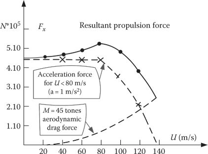
FIGURE 6.6 Typical propulsion force profile for a 45 ton high-speed MAGLEV.
To comply with Geo = 35 at 215 Hz, g = 10 mm, and dAl=4–6 mm, the equivalent secondary conductivity is (6.3)
As the aluminum electrical conductivity σAl ≈ 3.25 × 10⁷ (Ω m)−1, the concerted influence of edge effect and of solid back-iron saturation together with the counteracting effect of solid back-iron conductivity can corner the 2.96 electrical equivalent conductivity reduction ratio. A reduction of aluminum plate overhangs will contribute to bring the electrical conductivity into range; also a reduction of aluminum plate thickness dAl will produce similar effects but will also reduce the magnetization mmf, as added benefit.
The rather large slip S ≈ 0.07 at maximum speed (f2 = 15 Hz) is justified by the necessity to keep the dynamic end effect adverse influences on performance within practical limits. The design, from this point, may follow the path used for urban vehicles with SLIM propulsion. For typical results, see the examples in Chapters 3 and 4, for high-speed SLIMs (Figure 3.23).
6.4 Optimization Design of Slim: Urban Vehicles
The preliminary electromagnetic design methodologies developed in Chapter 5 should constitute a good ground for a closer to target initialization of the optimization design and the SLIM model required in this enterprise.
For optimization design, a few steps are appropriate:
Specifications and constraints
Variables vector
Cost (fitting) objective function
Development of an SLIM model (realistic, but still reasonable in terms of computer effort for its repeated usage in optimization process)
Choosing a mathematical optimization method (deterministic or evolutionary as for rotary machines [4])
Developing a computer code to easily handle the path from specifications to final design with ready-to-use documentation for manufacturing
A possible cost function may be
with
nSLIM as the number of SLIMs for the designated transportation system
Ca as the cost of active materials in an SLIM primary
Cf+ m as the cost of framing and manufacturing of an SLIM
Closses as the cost of losses in an SLIM for the entire operating life
Cinv as the inverter initial cost proportional to SLIM KVA (inversely proportional to SLIM efficiency and power factor)
as the cost of inverter losses for its operation life
Cmaint as the maintenance costs per one SLIM + its inverter for the entire operation life
Cseci as the initial secondary cost for entire track length
Csecmaint as the secondary maintenance cost for entire operation life
Typical constraints are related to costs or losses or both, but translated in terms of analytical SLIM model; they are efficiency x power factor of SLIM at base speed, primary winding maximum temperature or peak current for given dc power bus voltage and peak starting thrust and given peak thrust versus speed envelope or maximum normal force of SLIM, etc.
In Ref. [5], a thorough optimization design process for an SLIM-MAGLEV system with 33.3 kN peak thrust for vehicles that contain 6, 8, and 10 SLIM modules is introduced. The cost function in [5] has a multi-objective character but still less demanding than that of (6.41).
In short, the two main cost function options in [5] are related to efficiency and SLIM primary weight and, respectively, secondary material cost and SLIM primary weight. As expected, a better efficiency is accompanied by larger SLIM primary weight and lower secondary materials cost, while lower SLIM primary weight leads to notably lower efficiency; the power factor is smaller when efficiency is larger and vice versa. Efficiency below 64% and power factor below 0.647 are typical but not for the same optimal design, directed to SLIM-MAGLEVs at 200 km/h.
The results in previous paragraphs, based on the optimum goodness factor concept, suggest better performance than in [5] even at higher speed (up to 100 m/s), with track costs low but comparable to competitive solutions for wheeled vehicles or MAGLEVs. The reader is advised to proceed with care as the SLIM optimal design is far from an exhausted subject, even in the presence of a few commercial, urban, wheeled, successful SLIM vehicles.
6.5 Summary
By design, dimensioning (sizing) for given specifications is meant.
Transportation LIMs refer to urban and interurban people (or freight) movers on wheels or in MAGLEVs when dynamic end effect has to be considered [3,6].
In MAGLEV applications, the SLIMs are placed on both sides of the vehicles below (or even above) the track structure; in one case, the net normal force helps the magnetic suspension while in the other impedes on it; zero normal force SLIM slip frequency control leads to efficiency below 0.65, even for urban applications.
Only aluminum-on-iron long track secondary SLIMs are considered here practical, due to overall cost limitations.
1–3 pieces (laminations) may constitute the mild steel secondary back iron, to increase the field penetration depth and thus allow sufficient airgap flux density; also, for the same reason, the length of the primary pole pitch is limited to 0.22–0.27 m.
To allow tight curves in the track, the total length of the short primary on board should be below 2–2.75 m for urban applications and beyond 3.5 m/per unit in interurban applications.
Thus, the number of primary poles 2p + 1 = 7 ÷ 11(15) per unit.
2p + 1 poles with double-layer windings and half-filled end poles with chorded coils are recommended to reduce end-coil length and primary copper losses.
The mechanical airgap varies from 8 to 12 mm, and the aluminum sheet should be 4–6 mm thick.
The slip frequency should be in the range of 6–8 Hz in urban SLIM vehicles and 10–15 Hz in high-speed (interurban) vehicles, to provide enough thrust but also to reduce noise and vibration at start and dynamic end effect at maximum speed.
The key design concept used here is the optimum goodness factor Geo(f1max) (zero end effect thrust, at zero slip and maximum speed). For urban transportation, even Ge < Geo may be adopted for lower cost reasons.
(Geo)f1ma imposes 2(3) back-iron laminations in the secondary and a thickness hy2 ≤ 25 mm.
Peak thrust, Fxpeak (from zero to base speed), has to be obtained, eventually for (Geo)fr2 = 1 − 2; this is a key design verification.
Fxpeak leads to the peak phase current mmf w1I1peak and the peak airgap flux density Bg1max, both essential in designing the primary slots and back iron.
Then, the second verification is related to peak thrust at base speed and full voltage, which leads to the number of turns w1 per phase.
The third verification is related to thrust at peak speed at max. inverter voltage including (also at base speed) the end effect thrust, fe, or emf correction coefficient, Ke.
In the presence of dynamic end effect, it seems to be more practical to use the field theory and power balances to calculate performance for the entire speed range; only at the end, the circuit parameters are worth calculating to serve for the control system design.
Designing for optimum goodness factor brings the end effect deteriorating influence within limits, but new end effect compensation schemes (as discussed in Chapter 4) should not be left out, as addition for performance boosting.
Despite of the SLIM low power factor (below 0.6), which leads to inverter overratings, its ruggedness and around 75%–80% efficiency may be acceptable in the long run, for medium- and high-speed applications where initial cost is critical.
References
1. J.F. Gieras, Linear Induction Drives, Oxford University Press, Oxford, U.K., 1994.
2. I. Boldea, and S.A. Nasar, Linear Motion Electromagnetic Systems, Chapter 6, Wiley Interscience, New York, 1985.
3. T. Higuchi, T. Nishimoto, S. Nonaka, and H. Muramoto, Design optimization of single sided linear induction motors for MAGLEV vehicles, Record of LDIA-2001, Nagasaki, Japan, pp. 25–29.
4. I. Boldea and L. Tutelea, Electric Machines: Steady State Transients and Design with Matlab, CRC Press, Taylor & Francis, New York, 2009.
5. C. Cabral, L.J. Concalves, E. Pappalardo, and C. Cabrita, A new model and performance of SLIM taking into account the back iron saturation, Record of LDIA-1998, Tokyo, Japan, pp. 359–362.
6. S. Nonaka and T. Higuchi, Design strategy of SLIMs for propulsion of vehicles, Record of International Conference on MAGLEV & Linear Drives, IEEE, Las Vegas, NV, 1987, pp. 1–6.