7

Strategic lead-time management

Time-based competition

Customers in all markets, industrial or consumer, are increasingly time-sensitive.¹ In other words they value time and this is reflected in their purchasing behaviour. Thus, for example, in industrial markets buyers tend to source from suppliers with the shortest lead-times who can meet their quality specification at an acceptable price. In consumer markets, as we highlighted in Chapter 2, customers make their choice from amongst the brands available at the time; hence if the preferred brand is out-of-stock it is quite likely that a substitute brand will be purchased instead.

In the past it was often the case that price was paramount as an influence on the purchase decision. Now, whilst price is still important, a major determinant of choice of supplier or brand is the ‘cost of time’. The cost of time is simply the additional costs that a customer must bear whilst waiting for delivery or whilst seeking out alternatives.

There are many pressures leading to the growth of time-sensitive markets but perhaps the most significant are:

1. Shortening life cycles
2. Customers’ drive for reduced inventories
3. Volatile markets making reliance on forecasts dangerous

1 Shortening life cycles

The concept of the product life cycle is well established. It suggests that for many products there is a recognisable pattern of sales from launch through to final decline (see Figure 7.1).

Figure 7.1 The product life cycle

A feature of the last few decades has been the shortening of these life cycles. Take as an example the case of the typewriter. The early mechanical typewriter had a life cycle of about 30 years – meaning that an individual model would be little changed during that period. These mechanical typewriters were replaced by the electro-mechanical typewriter, which had a life cycle of approximately ten years. The electro-mechanical typewriter gave way to the electronic typewriter with a four-year life cycle. Now PCs, laptops and tablets have taken over with a life cycle of one year or less!

In situations like this, the time available to develop new products, to launch them and to meet marketplace demand is clearly greatly reduced. Hence the ability to ‘fast track’ product development, manufacturing and logistics becomes a key element of competitive strategy. Figure 7.2 shows the effect of being late into the market and slow to meet demand.

Figure 7.2 Shorter life cycles make timing crucial

However, it is not just time-to-market that is important. Once a product is on the market, the ability to respond quickly to demand is equally important. Here the lead-time to re-supply a market determines the organisation’s ability to exploit demand during the life cycle. It is apparent that those companies that can achieve reductions in the order-to-delivery cycle will have a strong advantage over their slower competitors.

2 Customers’ drive for reduced inventories

One of the most pronounced phenomena of recent years has been the almost universal move by companies to reduce their inventories. Whether the inventory is in the form of raw materials, components, work-in-progress or finished products, the pressure has been to release the capital locked up in stock and hence simultaneously to reduce the holding cost of that stock. The same companies that have reduced their inventories in this way have also recognised the advantage that they gain in terms of improved flexibility and responsiveness to their customers.

The knock-on effect of this development upstream to suppliers has been considerable. It is now imperative that suppliers can provide a JIT delivery service. Timeliness of delivery – meaning delivery of the complete order at the time required by the customer – becomes the number one order-winning criterion.

Many companies still think that the only way to service customers who require JIT deliveries is for them, the supplier, to carry the inventory instead of the customer. Whilst the requirements of such customers could always be met by the supplier carrying inventory close to the customer(s), this is simply shifting the cost burden from one part of the supply chain to another – indeed the cost may even be higher. Instead what is needed is for the supplier to substitute responsiveness for inventory whenever possible.

As we discussed in Chapter 6, responsiveness essentially is achieved through agility in the supply chain. Not only can customers be serviced more rapidly but the degree of flexibility offered can be greater and yet the cost should be less because the pipeline is shorter. Figure 7.3 demonstrates that agility can enable companies to break free of the classic trade-off between service and cost. Instead of having to choose between either higher service levels or lower costs, it is possible to have the best of both worlds.

Figure 7.3 Breaking free of the classic service/cost trade-off

The concept of lead-time

From the customer’s viewpoint there is only one lead-time: the elapsed time from order to delivery. Clearly this is a crucial competitive variable as more and more markets become increasingly time competitive. Nevertheless it represents only a partial view of lead-time. Just as important, from the supplier’s perspective, is the time it takes to convert an order into cash and, indeed, the total time that working capital is committed from when materials are first procured through to when the customer’s payment is received.

Let us examine both of these lead-time concepts in turn.

1 The order-to-delivery cycle

From a marketing point of view, the time taken from receipt of a customer’s order through to delivery (sometimes referred to as order cycle time (OCT)) is critical. In today’s JIT environment, short lead-times are a major source of competitive advantage. Equally important, however, is the reliability or consistency of that lead-time. It can actually be argued that reliability of delivery is more important than the length of the order cycle – at least up to a point – because the impact of a failure to deliver on time is more severe than the need to order further in advance. However, because, as we have seen, long lead-times require longer-term forecasts, then the pressure from the customer will continue to be for deliveries to be made in ever-shorter time-frames.

What are the components of OCT? Figure 7.4 highlights the major elements.

Figure 7.4 The order cycle

Source: Stock, J.R. and Lambert, D.M., Strategic Logistics Management, 2nd edition, Irwin, 1987

Each of these steps in the chain will consume time. Because of bottlenecks, inefficient processes and fluctuations in the volume of orders handled, there will often be considerable variation in the time taken for these various activities to be completed. The overall effect can lead to a substantial reduction in the reliability of delivery. As an example, Figure 7.5 shows the cumulative effect of variations in an order cycle which results in a range of possible cycle times from 5 days to 25 days.

Figure 7.5 Total order cycle with variability

In those situations where orders are not met from stock but may have to be manufactured, assembled or sourced from external vendors, then clearly lead-times will be even further extended, with the possibility of still greater variations in total order-to-delivery time. Figure 7.6 highlights typical activities in such extended lead-times.

2 The cash-to-cash cycle

As we have already observed, a basic concern of any organisation is ‘How long does it take to convert an order into cash?’ In reality the issue is not just how long it takes to process orders, raise invoices and receive payment, but also how long is the pipeline from the sourcing of raw material through to the finished product because throughout the pipeline resources are being consumed and working capital needs to be financed.

Figure 7.6 Lead-time components

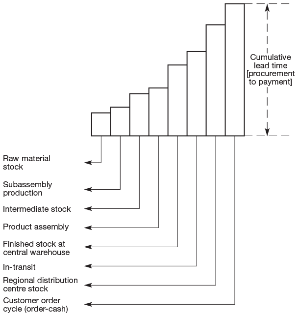
From the moment when decisions are taken on the sourcing and procurement of materials and components, through the manufacturing and assembly process to final distribution, time is being consumed. That time is represented by the number of days of inventory in the pipeline, whether as raw materials, work-in-progress, goods in transit, or time taken to process orders, issue replenishment orders, as well as time spent in manufacturing, time in queues or bottlenecks and so on. The control of this total pipeline is the true scope of logistics lead-time management. Figure 7.7 illustrates the way in which cumulative lead-time builds up from procurement through to payment.

As we shall see later in this chapter, the longer the pipeline from source of materials to the final user the less responsive to changes in demand the system will be. It is also the case that longer pipelines obscure the ‘visibility’ of end demand so that it is difficult to link manufacturing and procurement decisions to marketplace requirements. Thus we find an inevitable build-up of inventory as a buffer at each step along the supply chain. An approximate rule of thumb suggests that the amount of safety stock in a pipeline varies with the square root of the pipeline length.

Overcoming these problems and ensuring timely response to volatile demand requires a new and fundamentally different approach to the management of lead-times.

Figure 7.7 Strategic lead-time management

Logistics pipeline management

The key to the successful control of logistics lead-times is pipeline management. Pipeline management is the process whereby manufacturing and procurement lead-times are linked to the needs of the marketplace. At the same time, pipeline management seeks to meet the competitive challenge of increasing the speed of response to those market needs.

The goals of logistics pipeline management are:

• Lower costs
• Higher quality
• More flexibility
• Faster response times

The achievement of these goals is dependent upon managing the supply chain as an entity and seeking to reduce the pipeline length and/or to speed up the flow through that pipeline. In examining the efficiency of supply chains it is often found that many of the activities that take place add more cost than value. For example, moving a pallet into a warehouse, repositioning it, storing it and then moving it out, in all likelihood has added no value but has added considerably to the total cost.

Very simply, value-adding time is time spent doing something that creates a benefit for which the customer is prepared to pay. Thus we could classify manufacturing as a value-added activity as well as the physical movement of the product and the means of creating the exchange. The old adage ‘the right product in the right place at the right time’ summarises the idea of customer value-adding activities. Thus any activity that contributes to the achievement of that goal could be classified as value adding.

Conversely, non-value-adding time is time spent on an activity whose elimination would lead to no reduction of benefit to the customer. Some non-value-adding activities are necessary because of the current design of our processes but they still represent a cost and should be minimised.

The difference between value-adding time and non-value-adding time is crucial to an understanding of how logistics processes can be improved. Flowcharting supply chain processes is the first step towards understanding the opportunities that exist for improvements in productivity through re-engineering those processes.

Once processes have been flowcharted, the first step is to bring together the managers involved in those processes to debate and agree exactly which elements of the process can truly be described as value adding. Agreement may not easily be achieved as no one likes to admit that the activity they are responsible for does not actually add any value for customers.

The next step is to do a rough-cut graph, highlighting visually how much time is consumed in both non-value-adding and value-adding activities. Figure 7.8 shows a generic example of such a graph.

Figure 7.8 Which activities add cost and which add value?

Figure 7.9 shows an actual analysis for a pharmaceutical product where the total process time was 40 weeks and yet value was only being added for 6.2 per cent of that time.

It will be noted from this example that most of the value is added early in the process and hence the product is more expensive to hold as inventory. Furthermore, much of the flexibility is probably lost as the product is configured and/or packaged in specific forms early in that process. Figure 7.10 shows that this product started as a combination of three active ingredients but very rapidly became 25 SKUs because it was packaged in different sizes, formats, etc., and was then held in inventory for the rest of the time in the company’s pipeline.

An indicator of the efficiency of a supply chain is given by its throughput efficiency, which can be measured as:

Throughput efficiency can be as low as 10 per cent, meaning that most time spent in a supply chain is non-value-adding time.

Figure 7.11 shows how cost-adding activities can easily outstrip value-adding activities.

The challenge to pipeline management is to find ways in which the ratio of value-added to cost-added time in the pipeline can be improved. Figure 7.12 graphically shows the goal of strategic lead-time management: to compress the chain in terms of time consumption so that cost-added time is reduced. Focusing on those parts of the graph that are depicted horizontally (i.e. representing periods of time when no value is being added), enables opportunities for improvement to be identified.

Figure 7.9 Value added through time

Figure 7.10 Variety through time

Figure 7.11 Cost-added versus value-added time

Pipeline management is concerned with removing the blockages and the fractures that occur in the pipeline and which lead to inventory build-ups and lengthened response times. The sources of these blockages and fractures are such things as extended set-up and change-over times, bottlenecks, excessive inventory, sequential order processing and inadequate pipeline visibility.

To achieve improvement in the logistics process requires a focus upon the lead-time as a whole, rather than the individual components of that lead-time. In particular the interfaces between the components must be examined in detail. These interfaces provide fertile ground for logistics process re-engineering.

Figure 7.12 Reducing non-value-adding time improves service and reduces cost

Reducing logistics lead-time

Because companies have typically not managed well the total flow of materials and information that link the source of supply with the ultimate customer, what we often find is that there is an incredibly rich opportunity for improving the efficiency of that process.

In those companies that do not recognise the importance of managing the supply chain as an integrated system it is usually the case that considerable periods of time are consumed at the interfaces between adjacent stages in the total process and in inefficiently performed procedures.

Because no one department or individual manager has complete visibility of the total logistics process, it is often the case that major opportunities for time reduction across the pipeline as a whole are not recognised. One electronics company in Europe did not realise for many years that, although it had reduced its throughput time in the factory from days down to hours, finished inventory was still sitting in the warehouse for three weeks! The reason was that finished inventory was the responsibility of the distribution function, which was outside the concern of production management.

To enable the identification of opportunities for reducing end-to-end pipeline time, an essential starting point is the construction of a supply chain map.

A supply chain map is essentially a time-based representation of the processes and activities that are involved as the materials or products move through the chain. At the same time, the map highlights the time that is consumed when those materials or products are simply standing still, i.e. as inventory.

In these maps, it is usual to distinguish between ‘horizontal’ and ‘vertical’ time. Horizontal time is time spent in process. It could be in-transit time, manufacturing or assembly time, time spent in production planning or processing and so on. It may not necessarily be time when customer value is being created but at least something is going on. The other type of time is vertical time, which is time when nothing is happening and hence the material or product is standing still as inventory. No value is being added during vertical time, only cost.

The labels ‘horizontal’ and ‘vertical’ refer to the maps themselves where the two axes reflect process time and time spent as static inventory respectively. Figure 7.13 depicts such a map for the manufacture and distribution of men’s underwear.

From this map it can be seen that horizontal time is 60 days. In other words, the various processes of gathering materials, spinning, knitting, dyeing, finishing, sewing and so on take 60 days to complete from start to finish. This is important because horizontal time determines the time that it would take for the system to respond to an increase in demand. Hence, if there were to be a sustained increase in demand, it would take that long to ‘ramp up’ output to the new level. Conversely, if there was a downturn in demand then the critical measure is pipeline volume, i.e. the sum of both horizontal and vertical time. In other words, it would take 175 days to ‘drain’ the system of inventory. So in volatile fashion markets, for instance, pipeline volume is a critical determinant of business risk.

Pipeline maps can also provide a useful internal benchmark. Because each day of process time requires a day of inventory to ‘cover’ that day then, in an ideal world, the only inventory would be that needed to cover during the process lead-time. So a 60-day total process time would result in 60 days’ inventory. However, in the case highlighted here there are actually 175 days of inventory in the pipeline. Clearly, unless the individual processes are highly time variable or unless demand is very volatile, there is more inventory than can be justified.

It must be remembered that in multi-product businesses each product will have a different end-to-end pipeline time. Furthermore, where products comprise multiple components, packaging materials or sub-assemblies, total pipeline time will be determined by the speed of the slowest moving item or element in that product. Hence in procuring materials for and manufacturing a household aerosol air freshener, it was found that the replenishment lead-time for one of the fragrances used was such that weeks were added to the total pipeline.

Mapping pipelines in this way provides a powerful basis for logistics re-engineering projects. Because it makes the total process and its associated inventory transparent, the opportunities for reducing non-value-adding time become apparent. In many cases much of the non-value-adding time in a supply chain is there because it is self-inflicted through the ‘rules’ that are imposed or that have been inherited. Such rules include: economic batch quantities, economic order quantities, minimum order sizes, fixed inventory review periods, production planning cycles and forecasting review periods.

The importance of strategic lead-time management is that it forces us to challenge every process and every activity in the supply chain and to apply the acid test of ‘does this activity add value for a customer or consumer or does it simply add cost?’

The basic principle to be noted is that every hour of time in the pipeline is directly reflected in the quantity of inventory in the pipeline and thus the time it takes to respond to marketplace requirements.

Figure 7.13 Supply chain mapping – an example

Source: Reprinted with permission from Emerald Group Publishing Limited, originally published in Scott, C. and Westbrook, R., ‘New strategic tools for supply chain management’, International Journal of Physical Distribution of Logistics Management, 21(1) © Emerald Group Publishing 1991

A simple analogy is with an oil pipeline. Imagine a pipeline from a refinery to a port that is 500 kilometres long. In normal conditions there will be 500 kilometres equivalent of oil in the pipeline. If there is a change in requirement at the end of the pipeline (say, for a different grade of oil) then 500 kilometres of the original grade has to be pumped through before the changed grade reaches the point of demand.

In the case of the logistics pipeline, time is consumed not just in slow-moving processes but also in unnecessary stock holding – whether it be raw materials, work-in-progress, waiting at a bottleneck or finished inventory. By focusing on improving key supply chain processes companies can dramatically improve their competitiveness, as the case of Johnstons of Elgin (see box below) illustrates.

Reference

1. Stalk, G. and Hout, T.M., Competing Against Time, The Free Press, 1990.