CHAPTER 1

MATLAB Introduction and Working Environment

Introduction to Working with MATLAB

Whenever you use a program of this type, it is necessary to know the general characteristics of how the program interprets notation. This chapter will introduce you to some of the practices used in the MATLAB environment. If you are familiar with using MATLAB, you may wish to skip over this chapter.

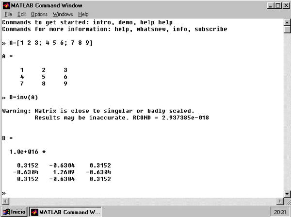
The best way to learn MATLAB is to use the program. Each example in the book consists of the header with the prompt for user input “>>” and the response from MATLAB appears on the next line. See Figure 1-1.

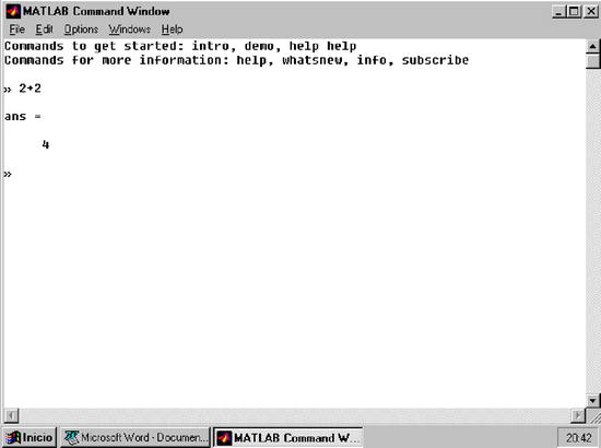
At other times, depending on the type of user input used, MATLAB returns the response using the expression “ans =”. See Figure 1-2.

In a program like MATLAB it is always necessary to pay attention to the difference between uppercase and lowercase letters, types of parentheses or square brackets, the amount of spaces used in your input and your choice of punctuation (e.g., commas, semicolons). Different uses will produce different results. We will go over the general rules now.

Any input to run MATLAB should be written to the right of the header (the prompt for user input “>>”). You then obtain the response in the lines immediately below the input.

When an input is proposed to MATLAB in the command window that does not cite a variable to collect the result, MATLAB returns the response using the expression ans=.

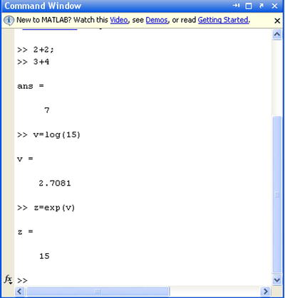
If at the end of the input we put a semicolon, the program runs the calculation(s) and keeps them in memory (Workspace), but does not display the result on the screen (see the first input in Figure 1-3 as an example).

The input prompt appears “>> ” to indicate that you can enter a new entry.

If you enter and define a variable that can be calculated, you can then use that variable as the argument for subsequent entries. This is the case for the variable v in Figure 1-3, which is subsequently used as an input in the exponential function.

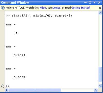
Like the C programming language, MATLAB is sensitive to the difference between uppercase and lowercase letters; for example, “Sin (x)” is different from “sin (x)”. The names of all built-in functions begin with lowercase. There should be no spaces in the names of symbols of more than one letter or in the names of functions. In other cases, spaces are simply ignored. They can be used in some cases to make input more readable. Multiple entries in the same line of command, separated by commas, can also be used. In this case, press Enter at the end of the last entry (see Figure 1-4). If you use a semicolon at the end of one of the entries of the line, as we stated before, its corresponding output is ignored.

It is possible to enter descriptive comments in a command input line by starting the comment with the “%” sign. When you run the input, MATLAB ignores the rest of the line to the right of the % sign:

>> L = log (123) % L is a natural logarithm
L =
         4.8122
>>

To simplify the introduction of a script to be evaluated by the MATLAB interpreter (via the command window), you can use the arrow computer keys. For example, if you press the up arrow once, MATLAB will recover the last entry submitted in MATLAB. If you press the up arrow key twice, MATLAB recovers the prior entry submitted, and so on. This can save you the headache of re-entering complicated formulae.

Similarly, if you type a sequence of characters in the input area and then click the up arrow, MATLAB recovers the last entry that begins with the specified string.

Commands entered during a MATLAB session are temporarily stored in the buffer (Workspace) until you end the session with the program, at which time they can be permanently stored in a file or you lose them permanently.

Below is a summary of the keys that can be used in the input area of MATLAB (command line), as well as their functions:

The command clc clears the command window, but does not delete the content of the Workspace (that content remains in memory).

Numerical Calculations with MATLAB

You can use MATLAB as a powerful numerical calculator. Most calculators handle numbers only with a preset degree of precision, however MATLAB performs exact calculations with the necessary precision. In addition, unlike calculators, we can perform operations not only with individual numbers, but also with objects such as arrays.

Most of the themes in classical numerical calculations, are treated in this software. It supports matrix calculations, statistics, interpolation, fit by least squares, numerical integration, minimization of functions, linear programming, numerical algebraic and resolution of differential equations and a long list of processes of numerical analysis that we’ll see later in this book.

Here are some examples of numerical calculations with MATLAB. (As we all know, for results it is necessary to press Enter once you have written the corresponding expressions next to the prompt “>>”)

We can simply calculate 4 + 3 and get as a result 7. To do this, just type 4 + 3, and then Enter.

>> 4 + 3

Ans =

7

Also we can get the value of 3 to the 100th power, without having previously set the level of precision. For this purpose press 3 ^ 100.

>> 3 ^ 100

Ans =

5. 1538e + 047

You can use the command “format long e” to pass the result of the operation with 16 digits before the exponent (scientific notation).

>> format long e

>> 3 ^ 100

ans =

5.153775207320115e+047

We can also work with complex numbers. We will get the result of the operation (2 + 3i) raised to the 10th power, by typing the expression (2 + 3i) ^ 10.

>> (2 + 3i) ^ 10

Ans =

-1. 415249999999998e + 005 - 1. 456680000000000e + 005i

The previous result is also available in short format, using the “format short” command.

>> format short
>> (2 + 3i) ^ 10

ans =

-1.4152e+005- 1.4567e+005i

Also we can calculate the value of the Bessel function found for 11.5. To do this type Besselj (0,11.5).

>> besselj(0, 11.5)

ans =

   -0.0677

Symbolic Calculations with MATLAB

MATLAB handles symbolic mathematical computation, manipulating formulae and algebraic expressions easily and quickly and can perform most operations with them. You can expand, factor and simplify polynomials, rational and trigonometric expressions, you can find algebraic solutions of polynomial equations and systems of equations, can evaluate derivatives and integrals symbolically, and find function solutions for differential equations, you can manipulate powers, limits and many other facets of algebraic mathematical series.

To perform this task, MATLAB requires all the variables (or algebraic expressions) to be written between single quotes to distinguish them from numerical solutions. When MATLAB receives a variable or expression in quotes, it is considered symbolic.

Here are some examples of symbolic computation with MATLAB.

1. Raise the following algebraic expression to the third power: (x + 1) (x+2)-(x+2) ^ 2. This is done by typing the following expression: expand (‘((x + 1) (x+2) - (x+2) ^ 2) ^ 3’). The result will be another algebraic expression:

   >> syms x; expand (((x + 1) *(x + 2)-(x + 2) ^ 2) ^ 3)
   
   Ans =
   
   -x ^ 3-6 * x ^ 2-12 * x-8

   Note in this example, the syms x which is needed to initiate the variable x.

   You can then factor the result of the calculation in the example above by typing: factor (‘((x + 1) *(x + 2)-(x + 2) ^ 2) ^ 3’)

   >> syms x; factor(((x + 1)*(x + 2)-(x + 2)^2)^3)
   
   ans =
   
   -(x+2)^3

2. You can resolve the indefinite integral of the function (x ^ 2) sine (x) ^ 2 by typing: int (‘x ^ 2 * sin (x) ^ 2’, ‘x’)

   >> int('x^2*sin(x)^2', 'x')
   
   ans =
   
   x ^ 2 * (-1/2 * cos (x) * sin (x) + 1/2 * x)-1/2 * x * cos (x) ^ 2 + 1/4 * cos (x) * sin (x) + 1/4 * 1/x-3 * x ^ 3

   You can simplify the previous result:

   >> syms x; simplify(int(x^2*sin(x)^2, x))
   
   ans =
   
   sin(2*x)/8 - (x*cos(2*x))/4 - (x^2*sin(2*x))/4 + x^3/6

   You can express the previous result with more elegant mathematical notation:

   >> syms x; pretty(simplify(int(x^2*sin(x)^2, x)))
   
                         2             3
     sin(2 x)   x cos(2 x)   x  sin(2 x)   x
    -------- - ---------- - ----------- + --
        8           4             4        6

3. We can solve the equation 3ax-7 x ^ 2 + x ^ 3 = 0 (where a, is a parameter):

   >> solve('3*a*x-7*x^2 + x^3 = 0', 'x')
   
   ans =
   
   [                       0]
   [7/2+1/2 *(49-12*a)^(1/2)]
   [7/2-1/2 *(49-12*a)^(1/2)]

4. We can find the five solutions of the equation x ^ 5 + 2 x + 1 = 0:

   ans =
   
                                          -0.48638903593454300001655725369801
      0.94506808682313338631496614476119 + 0.85451751443904587692179191887616*i
      0.94506808682313338631496614476119 - 0.85451751443904587692179191887616*i
    - 0.70187356885586188630668751791218 - 0.87969719792982402287026727381769*i
    - 0.70187356885586188630668751791218 + 0.87969719792982402287026727381769*i

On the other hand, MATLAB may use the libraries of the Maple V program to work with symbolic math and can thus extend its field of application. In this way, you can use MATLAB to work on problems in areas including differential forms, Euclidean geometry, projective geometry, statistics, etc.

At the same time, you also can expand your options for numerical calculations using the libraries from MATLAB and libraries of Maple (combinatorics, optimization, theory of numbers, etc.).

Graphics with MATLAB

MATLAB produces graphs of two and three dimensions, as well as outlines and graphs of density. You can represent both the graphics and list the data in MATLAB. MATLAB allows you to control colors, shading and other graphics features, and also supports animated graphics. Graphics produced by MATLAB are portable to other programs.

Here are some examples of MATLAB graphics:

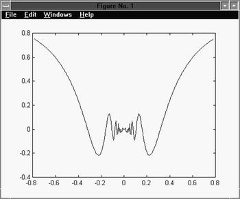
1. You can represent the function xsine (x) for x ranging between -π/4 and π/4, using 300 equidistant points for the intervals. See Figure 1-5.

   >> x = linspace(-pi/4,pi/4,300);
   >> y = x.*sin(1./x);
   >> plot(x,y)

   

   Figure 1-5.

   Note the dots (periods) in this example in the second line. These are not decimal points and should not be confused as such. These indicate that if you are working with vectors or matrices that the following operator needs to be applied to every element of the vector or matrix. For an easy example, let’s use x .*3. If x is a matrix, then all elements of x should be multiplied by 3. Again, be careful to avoid confusion with decimal points. It is sometimes wise to represent .6 as 0.6, for instance.

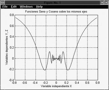
2. You can add the options frame and grille to the graph above, as well as create your own chart title and labels for axes. See Figure 1-6.

   >> x = linspace(-pi/4,pi/4,300);
   >> y = x.*sin(1./x);
   >> plot(x,y);
   >> grid;
   >> xlabel('Independent variable X'),
   >> ylabel ('Independent variable Y'),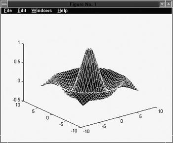
   >> title ('The functions y=sin(1/x)')

   

   Figure 1-6.

3. You can generate a graph of the surface for the function z = sine (sqrt(x^2+y^2)) /sqrt(x^2+y^2), where x and y vary over the interval (- 7.5, 7.5), taking equally spaced points in 5 tenths. See Figure 1-7.

   >> x =-7.5: .5:7.5;
   >> y = x;
   >> [X, Y] = meshgrid(x,y);
   >> Z = sin(sqrt(X.^2+Y.^2))./sqrt(X.^2+Y.^2);
   >> surf (X, Y, Z)

   

   Figure 1-7.

   In the first line of this example, note that the range is specified using colons. We did not use 0.5 and you can see that it can make the input somewhat confusing to a reader.

   These 3D graphics allow you to get an idea of the figures in space, and are very helpful in visually identifying intersections between different bodies, generation of developments of all kinds and volumes of revolution.

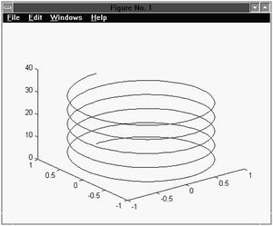
4. You can generate a three dimensional graphic corresponding to the helix in parametric coordinates: x = sine (t), y = cosine (t), z = t. See Figure 1-8.

   >> t = 0:pi/50:10*pi;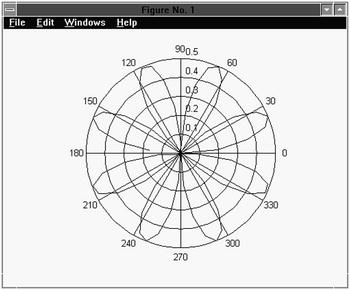
   >> plot3(sin(t),cos(t),t)

   

   Figure 1-8.

   We can represent a planar curve given by its polar coordinates r = cosine (2t) * sine (2t) for t varying between 0 and 2π, taking equally spaced points in one-hundredths of the considered range. See Figure 1-9.

   >> t = 0:.01:2 * pi;
   >> r = sin(2*t).* cos(2*t);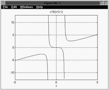
   >> polar(t,r)

   

   Figure 1-9.

5. We can also make a graph of a function considered as symbolic, using the command “ezplot”. See Figure 1-10.

   >> y ='x ^ 3 /(x^2-1)';
   >> ezplot(y,[-5,5])

In the corresponding chapter on graphics we will extend these concepts.

MATLAB and Programming

By properly combining all the objects defined in MATLAB appropriate to the work rules defined in the program, you can build useful mathematical research programming code. Programs usually consist of a series of instructions in which values are calculated, assigned a name and are reused in further calculations.

As in programming languages like C or Fortran, in MATLAB you can write programs with loops, control flow and conditionals. In MATLAB you can write procedural programs, (i.e., to define a sequence of standard steps to run). As in C or Pascal, a Do, For, or While loop may be used for repetitive calculations. The language of MATLAB also includes conditional constructs such as If Then Else. MATLAB also supports logic functions, such as And, Or, Not and Xor.

MATLAB supports procedural programming (iterative, recursive, loops…), functional programming and object-oriented programming. Here are two simple examples of programs. The first generates the order n Hilbert matrix, and the second calculates the Fibonacci numbers.

% Generating the order n Hilbert matrix
t = '1/(i+j-1)';
for i = 1:n
for j = 1:n
a(i,j) = eval(t);
end
end

% Calculating Fibonacci numbers
f = [1 1]; i = 1;
while f(i) + f(i-1) < 1000
f(i+2) = f(i) + f(i+1);
i = i+1
end