
![]()
Complex Numbers and Functions of Complex Variables
Complex Numbers
Complex numbers are easily implemented in MATLAB in standard binary form a+bi or a+bj, where the symbol i or j represents the imaginary unit. It is not necessary to include the product symbol (the asterisk) before the imaginary unit, but if it is included, everything will still work correctly. However, it is important that spaces are not introduced between the imaginary unit and its coefficient.
A complex number can have a symbolic real or imaginary part, and operations on complex numbers can be carried out in any mode of precision that is set with the command format. Therefore, it is possible to work with complex numbers in exact rational format via the command format rat.
The common operations (sum, difference, product, division and exponentiation) are carried out on complex numbers in the usual way. Examples are shown in Figure 3-1.

Obviously, as the real numbers are a subset of the complex numbers, a function of complex variables will also be valid for real variables.
General Functions of Complex Variables
MATLAB has a range of preset general functions of complex variables, which of course will also be valid for integer, rational, and real variables. The most important functions are presented in the following sections.
Trigonometric Functions of a Complex Variable
Below is a table of the trigonometric functions of a complex variable and their inverses that MATLAB incorporates, illustrated with examples.
|
Function |
Inverse |
|---|---|
|
sin (z) sine >> sin(5-6i) ans = -1 9343e + 002-5 7218e + 001i |
asin(z) arcsine >> asin(1-i) ans = 0.6662 - 1.0613i |
|
cos (z) cosine >> cos(3 + 4i) ans = -27.0349 - 3.8512i |
acos (z) arccosine >> acos(-i) ans = 1.5708 + 0.8814i |
|
tan (z) tangent >> tan(pi/4i) ans = 0 - 0.6558i |
atan(z) and atan2(z) arctangent >> atan(-pi*i) ans = 1.5708 - 0.3298i |
|
csc (z) inverse cosecant >> csc(1-i) ans = 0.6215 + 0.3039i |
acsc (z) arccosecant >> acsc(2i) ans = 0 - 0.4812i |
|
sec (z) secant >> sec(-i) ans = 0.6481 |
asec (z) arcsecant >> asec(0.6481+0i) ans = 0 + 0.9999i |
|
cot (z) cotangent >> cot(-j) ans = 0 + 1.3130i |
acot (z) arccotangent >> acot(1-6j) ans = 0.0277 + 0.1635i |
Hyperbolic Functions of a Complex Variable
Below is a table of the hyperbolic functions of a complex variable and their inverses that MATLAB incorporates, illustrated with examples.
|
Function |
Inverse |
|---|---|
|
sinh(z) hyperbolic sine >> sinh(1+i) ans = 0.6350 + 1.2985i |
asinh(z) arc hyperbolic sine >> asinh(0.6350 + 1.2985i) ans = 1.0000 + 1.0000i |
|
cosh(z) hyperbolic cosine >> cosh(1-i) ans = 0.8337 - 0.9889i |
acosh(z) arc hyperbolic cosine >> acosh(0.8337 - 0.9889i) ans = 1.0000 - 1.0000i |
|
tanh(z) hyperbolic tangent >> tanh(3-5i) ans = 1.0042 + 0.0027i |
atanh(z) arc hyperbolic tangent >> atanh(3-41) ans = -0.0263 - 1.5708i |
|
csch(z) hyperbolic cosecant >> csch(i) ans = 0 - 1.1884i |
acsch (z) arc hyperbolic cosecant >> acsch(- 1.1884i) ans = 0 + 1.0000i |
|
sech(z) hyperbolic secant >> sech(i^i) ans= 0.9788 |
asech(z) arc hyperbolic secant >> asech(5-0i) ans = 0 + 1.3694i |
|
coth(z) hyperbolic cotangent >> coth(9+i) ans = 1.0000 - 0.0000i |
acoth(z) arc hyperbolic cotangent >> acoth(1-i) ans = 0.4024 + 0.5536i |
Exponential and Logarithmic Functions of a Complex Variable
Below is a table of exponential and logarithmic functions that MATLAB incorporates, illustrated with examples.
|
Function |
Meaning |
|---|---|
|
exp (z) |
Base e exponential function (e ^ x) >> exp(1-i) ans = 1.4687 - 2.2874i |
|
log (x) |
Base e logarithm >> log(1.4687-2.2874i) ans = 1.0000 - 1.0000i |
|
log10 (x) |
Base 10 logarithm >> log10 (100 + 100i) ans = 2.1505 + 0.3411i |
|
log2 (x) |
Base 2 logarithm >> log2(4-6i) ans = 2.8502 - 1.4179i |
|
pow2 (x) |
Base 2 power function >> pow2(2.8502-1.4179i) ans = 3.9998 - 6.0000i |
|
sqrt (x) |
Square root >> sqrt(1+i) ans = 1.0987 + 0.4551i |
Specific Functions of a Complex Variable
MATLAB incorporates a group of functions specifically to work with moduli, arguments, and real and imaginary parts of complex numbers. Among these are the following:
|
Function |
Meaning |
|---|---|
|
abs (Z) |
The modulus (absolute value) of Z >> abs(12.425-8.263i) ans = 14.9217 |
|
angle (Z) |
The argument of Z >> angle(12.425-8.263i) ans = -0.5869 |
|
conj (Z) |
The complex conjugate of Z >> conj(12.425-8.263i) ans = 12.4250 + 8.2630i |
|
real (Z) |
The real part of Z >> real(12.425-8.263i) ans = 12.4250 |
|
imag (Z) |
The imaginary part of Z >> imag(12.425-8.263i) ans = -8.2630 |
|
floor (Z) |
Applies the floor function to real(Z) and imag(Z) >> floor(12.425-8.263i) ans = 12.0000 - 9.0000i |
|
ceil (Z) |
Applies the ceil function to real(Z) and imag(Z) >> ceil(12.425-8.263i) ans = 13.0000 - 8.0000i |
|
round (Z) |
Applies the round function to real(Z) and imag(Z) >> round(12.425-8.263i) ans = 12.0000 - 8.0000i |
|
fix (Z) |
Applies the fix function to real(Z) and imag(Z) >> fix(12.425-8.263i) ans = 12.0000 8.0000i |
Basic Functions with a Complex Vector Argument
MATLAB enables you to work with complex matrices and vector functions. We must not forget that these functions are also valid for real variables, since the real numbers are a special case of the complex numbers, being complex numbers with zero imaginary part. Below is a table summarizing the specific functions of a complex vector that MATLAB offers. Later, when we tabulate the functions of a complex matrix variable, we will observe that all of them are also valid for vector variables, a vector being a particular case of a matrix.
|
max (V) |
Maximum component (for complex vectors the max is calculated as the component with maximum absolute value) >> max([1-i 1+i 3-5i 6i]) ans = 0 + 6.0000i >> max([1, 0, -23, 12, 16]) ans = 16 |
|
min (V) |
Minimum component (for complex vectors the min is calculated as the component with minimum absolute value) >> min([1-i 1+i 3-5i 6i]) ans = 1.0 - 1.0000i >> min([1, 0, -23, 12, 16]) ans = -23 |
|
mean (V) |
Arithmetic mean of the components of V >> mean([1-i 1+i 3-5i 6i]) ans = 1.2500 + 0.2500i >> mean([1, 0, -23, 12, 16]) ans = 1.2000 |
|
median (V) |
Median of the components of V >> median([1-i 1+i 3-5i 6i]) ans = 2.0000 2.0000i >> median([1, 0, - 23, 12, 16]) ans = 1 |
|
std (V) |
Standard deviation of the components of V >> std([1-i 1+i 3-5i 6i]) ans = 4.7434 >> std([1, 0, -23, 12, 16]) ans = 15.1888 |
|
sort (V) |
Sorts the components of V in ascending order. For complex vectors the order is determined by the absolute values of the components. >> sort([1-i 1+i 3-5i 6i]) ans = Columns 1 through 2 1.0000 - 1.0000i 1.0000 + 1.0000i Columns 3 through 4 3.0000 - 5.0i 6.0000i >> sort([1, 0, -23, 12, 16]) ans = -23 0 1 12 16 |
|
sum (V) |
Sums the components of V >> sum([1-i 1+i 3-5i 6i]) ans = 5.0000 + 1.0000i >> sum([1, 0, -23, 12, 16]) ans = 6 |
|
prod (V) |
Finds the product of the elements of V, so n!= prod(1:n) >> prod([1-i 1+i 3-5i 6i]) ans = 60.0000 + 36.0000i >> prod([1, 0, -23, 12, 16]) ans = 0 |
|
cumsum (V) |
Gives the cumulative sums of V >> cumsum([1-i 1+i 3-5i 6i]) ans = Columns 1 through 2 1.0000 - 1.0000i 2.0000 Columns 3 through 4 5.0000 - 5.0000i 5.0000 + 1.0000i >> cumsum([1, 0, -23, 12, 16]) ans = 1 1 -22 -10 -6 |
|
cumprod (V) |
Gives the cumulative products of V >> cumprod([1-i 1+i 3-5i 6i]) ans = Columns 1 through 2 1.0000 - 1.0000i 2.0000 Columns 3 through 4 6.0000 - 10.0000i 60.0000 + 36.0000i >> cumprod([1, 0, -23, 12, 16]) ans = 1 0 0 0 0 |
|
diff (V) |
Gives the vector of first differences of the components of V (Vt - Vt-1) >> diff([1-i 1+i 3-5i 6i]) ans = 0 + 2.0000i 2.0000 - 6.0000i -3.0000 + 11.0000i >> diff([1, 0, -23, 12, 16]) ans = -1 -23 35 4 |
|
gradient (V) |
Gives the gradient of V > gradient([1-i 1+i 3-5i 6i]) ans = Columns 1 through 3 0 + 2.0000i 1.0000 - 2.0000i -0.5000 + 2.5000i Column 4 -3.0000 + 11.0000i >> gradient([1, 0, -23, 12, 16]) ans = -1.0000 -12.0000 6.0000 19.5000 4.0000 |
|
del2 (V) |
Gives the Laplacian of V (5-point discrete) >> del2([1-i 1+i 3-5i 6i]) ans = Columns 1 through 3 2.2500 - 8.2500i 0.5000 - 2.0000i -1.2500 + 4.2500i Column 4 -3.0000 + 10.5000i >> del2 ([1, 0, -23, 12, 16]) ans = -25.5000 -5.5000 14.5000 -7.7500 -30.0000 |
|
fft (V) |
Returns the discrete Fourier transform of V >> fft([1-i 1+i 3-5i 6i]) ans = Columns 1 through 3 5.0000 + 1.0000i -7.0000 + 3.0000i 3.0000 - 13.0000i Column 4 3.0000 + 5.0000i >> fft([1, 0, -23, 12, 16]) ans = Columns 1 through 3 6.0000 14.8435 + 35.7894i -15.3435 - 23.8824i Columns 4 through 5 -15.3435 + 23.8824i 14.8435 - 35.7894i |
|
fft2 (V) |
Returns the two-dimensional discrete Fourier transform of V >> fft2([1-i 1+i 3-5i 6i]) ans = Columns 1 through 3 5.0000 + 1.0000i -7.0000 + 3.0000i 3.0000 - 13.0000i Column 4 3.0000 + 5.0000i >> fft2([1, 0, -23, 12, 16]) ans = Columns 1 through 3 6.0000 14.8435 + 35.7894i -15.3435 - 23.8824i Columns 4 through 5 -15.3435 + 23.8824i 14.8435 - 35.7894i |
|
ifft (V) |
Returns the inverse discrete Fourier transform of V >> ifft([1-i 1+i 3-5i 6i]) ans = Columns 1 through 3 1.2500 + 0.2500i 0.7500 + 1.2500i 0.7500 - 3.2500i Column 4 -1.7500 + 0.7500i >> ifft([1, 0, -23, 12, 16]) ans = Columns 1 through 3 1.2000 2.9687 - 7.1579i -3.0687 + 4.7765i Columns 4 through 5 -3.0687 - 4.7765i 2.9687 + 7.1579i |
|
ifft2 (V) |
Returns the inverse two dimensional discrete Fourier transform of V >> ifft2([1-i 1+i 3-5i 6i]) ans = Columns 1 through 3 1.2500 + 0.2500i 0.7500 + 1.2500i 0.7500 - 3.2500i Column 4 -1.7500 + 0.7500i >> ifft2([1, 0, -23, 12, 16]) ans = Columns 1 through 3 1.2000 2.9687 - 7.1579i -3.0687 + 4.7765i Columns 4 through 5 -3.0687 - 4.7765i 2.9687 + 7.1579i |
Basic Functions with a Complex Matrix Argument
The functions described in the above table also support as an argument a complex matrix Z, in which case the result is a row vector whose components are the results of applying the function to each column of the matrix. Let us not forget that these functions are also valid for real variables.
|
max (Z) |
Returns a vector indicating the maximal components of each column of the matrix Z (for complex matrices the maximum is determined by the absolute values of the components) >> Z=[1-i 3i 5;-1+i 0 2i;6-5i 8i -7] Z = 1.0000 - 1.0000i 0 + 3.0000i 5.0000 -1.0000 + 1.0000i 0 0 + 2.0000i 6.0000 - 5.0000i 0 + 8.0000i -7.0000 >> Z=[1-i 3i 5-12i;-1+i 0 2i;6-5i 8i -7+6i] Z = 1.0000 - 1.0000i 0 + 3.0000i 5.0000 - 12.0000i -1.0000 + 1.0000i 0 0 + 2.0000i 6.0000 - 5.0000i 0 + 8.0000i -7.0000 + 6.0000i ans = 6.0000 - 5.0000i 0 + 8.0000i 5.0000 - 12.0000i >> Z1=[1 3 5;-1 0 2;6 8 -7] Z1 = 1 3 5 -1 0 2 6 8 -7 >> max(Z1) ans = 6 8 5 |
|
min (Z) |
Returns a vector indicating the minimal components of each column of the matrix Z (for complex matrices the minimum is determined by the absolute values of the components) >> min(Z) ans = 1.0000 - 1.0000i 0 0 + 2.0000i >> min(Z1) ans = -1 0 -7 |
|
mean (Z) |
Returns the vector of arithmetic means of the columns of the matrix Z >> mean(Z) ans = 2.0000 - 1.6667i 0 + 3.6667i -0.6667 - 1.3333i >> mean(Z1) ans = 2.0000 3.6667 0 |
|
median (Z) |
Returns the vector of medians of the columns of the matrix Z >> median(Z) ans = -1.0000 + 1.0000i 0 + 3.0000i -7.0000 + 6.0000i >> median(Z1) ans = 1 3 2 |
|
std (Z) |
Returns the vector of standard deviations of the columns of the matrix Z >> std(Z) ans = 4.7258 4.0415 11.2101 >> std(Z1) ans = 3.6056 4.0415 6.2450 |
|
sort (Z) |
Sorts in ascending order the components of the columns of Z. For complex matrices the ordering is by absolute value >> sort(Z) ans = 1.0000 - 1.0000i 0 0 + 2.0000i -1.0000 + 1.0000i 0 + 3.0000i -7.0000 + 6.0000i 6.0000 - 5.0000i 0 + 8.0000i 5.0000 - 12.0000i >> sort(Z1) ans = -1 0 -7 1 3 2 6 8 5 |
|
sum (Z) |
Returns the sum of the components of the columns of the matrix Z >> sum(Z) ans = 6.0000 - 5.0000i 0 + 11.0000i -2.0000 - 4.0000i >> sum(Z1) ans = 6 11 0 |
|
prod (Z) |
Returns the vector of products of the elements of the columns of the matrix Z >> prod(Z) ans = 1.0e+002 * 0.1000 + 0.1200i 0 -2.2800 + 0.7400i >> prod(Z1) ans = -6 0 -70 |
|
cumsum (Z) |
Gives the matrix of cumulative sums of the columns of Z >> cumsum(Z) ans = 1.0000 - 1.0000i 0 + 3.0000i 5.0000 - 12.0000i 0 0 + 3.0000i 5.0000 - 10.0000i 6.0000 - 5.0000i 0 + 11.0000i -2.0000 - 4.0000i >> cumsum(Z1) ans = 1 3 5 0 3 7 6 11 0 |
|
cumprod (V) |
Returns the cumulative products of the columns of the matrix Z >> cumprod(Z) ans = 1.0e+002 * 0.0100 - 0.0100i 0 + 0.0300i 0.0500 - 0.1200i 0 + 0.0200i 0 0.2400 + 0.1000i 0.1000 + 0.1200i 0 -2.2800 + 0.7400i >> cumprod(Z1) ans = 1 3 5 -1 0 10 -6 0 -70 |
|
diff (Z) |
Returns the matrix of first differences of the components of the columns of Z >> diff(Z) ans = -2.0000 + 2.0000i 0 - 3.0000i -5.0000 + 14.0000i 7.0000 - 6.0000i 0 + 8.0000i -7.0000 + 4.0000i >> diff(Z1) ans = -2 -3 -3 7 8 -9 |
|
gradient (Z) |
Returns the matrix of gradients of the columns of Z >> gradient(Z) ans = -1.0000 + 4.0000i 2.0000 - 5.5000i 5.0000 - 15.0000i 1.0000 - 1.0000i 0.5000 + 0.5000i 0 + 2.0000i -6.0000 + 13.0000i -6.5000 + 5.5000i -7.0000 - 2.0000i >> gradient(Z1) ans = 2.0000 2.0000 2.0000 1.0000 1.5000 2.0000 2.0000 –6.5000 -15.0000 |
|
del2 (V) |
Returns the discrete Laplacian of the columns of the matrix Z >> del2(Z) ans = 3.7500 - 6.7500i 1.5000 - 2.0000i 1.0000 - 7.2500i 2.0000 - 1.2500i -0.2500 + 3.5000i -0.7500 - 1.7500i 2.0000 - 5.7500i -0.2500 - 1.0000i -0.7500 - 6.2500i >> del2(Z1) ans = 2.2500 2.7500 -1.5000 2.5000 3.0000 -1.2500 -2.0000 -1.5000 -5.7500 |
|
fft (Z) |
Returns the discrete Fourier transform of the columns of the matrix Z >> fft(Z) ans = 6.0000 - 5.0000i 0 + 11.0000i -2.0000 - 4.0000i 3.6962 + 7.0622i -6.9282 - 1.0000i 5.0359 - 22.0622i -6.6962 - 5.0622i 6.9282 - 1.0000i 11.9641 - 9.9378i >> fft(Z1) ans = 6.0000 11.0000 0 -1.5000 + 6.0622i -1.0000 + 6.9282i 7.5000 - 7.7942i -1.5000 - 6.0622i -1.0000 - 6.9282i 7.5000 + 7.7942i |
|
fft2 (Z) |
Returns the two-dimensional discrete Fourier transform of the columns of the matrix Z >> fft2(Z) ans = 4.0000 + 2.0000i 19.9904 - 10.2321i -5.9904 - 6.7679i 1.8038 - 16.0000i 22.8827 + 28.9545i -13.5981 + 8.2321i 12.1962 - 16.0000i -8.4019 + 4.7679i -23.8827 - 3.9545i >> fft2(Z1) ans = 17.0000 0.5000 - 9.5263i 0.5000 + 9.5263i 5.0000 + 5.1962i 8.0000 + 13.8564i -17.5000 - 0.8660i 5.0000 - 5.1962i -17.5000 + 0.8660i 8.0000 - 13.8564i |
|
ifft (Z) |
Returns the inverse discrete Fourier transforms of the columns of the matrix Z >> ifft(Z) ans = 2.0000 - 1.6667i 0 + 3.6667i -0.6667 - 1.3333i -2.2321 - 1.6874i 2.3094 - 0.3333i 3.9880 - 3.3126i 1.2321 + 2.3541i -2.3094 - 0.3333i 1.6786 - 7.3541i >> ifft(Z1) ans = 2.0000 3.6667 0 -0.5000 - 2.0207i -0.3333 - 2.3094i 2.5000 + 2.5981i -0.5000 + 2.0207i -0.3333 + 2.3094i 2.5000 - 2.5981i |
|
ifft2 (Z) |
Returns the inverse two dimensional discrete Fourier transform of the columns of the matrix Z >> ifft2(Z) ans = 0.4444 + 0.2222i -0.6656 - 0.7520i 2.2212 - 1.1369i 1.3551 - 1.7778i -2.6536 - 0.4394i -0.9335 + 0.5298i 0.2004 - 1.7778i -1.5109 + 0.9147i 2.5425 + 3.2172i >> ifft2(Z1) ans = 1.8889 0.0556 + 1.0585i 0.0556 - 1.0585i 0.5556 - 0.5774i 0.8889 - 1.5396i -1.9444 + 0.0962i 0.5556 + 0.5774i -1.9444 - 0.0962i 0.8889 + 1.5396i |
General Functions with a Complex Matrix Argument
MATLAB incorporates a broad group of hyperbolic, trigonometric, exponential and logarithmic functions that support a complex matrix as an argument. Obviously, these functions also accept a complex vector as the argument, since a vector is a particular case of a matrix. All functions are applied element-wise to the matrix.
Trigonometric Functions of a Complex Matrix Variable
Below is a table of the trigonometric functions of a complex variable and their inverses that MATLAB incorporates, illustrated with examples. In the examples, the matrices Z and Z1 are those introduced in the first example concerning the sine function.
|
Trigonometric Functions |
|---|
|
sin(z) sine function >> Z=[1-i, 1+i, 2i;3-6i, 2+4 i, -i;i,2i,3i] Z = 1.0000 - 1.0000i 1.0000 + 1.0000i 0 + 2.0000i 3.0000 - 6.0000i 2.0000 + 4.0000i 0 - 1.0000i 0 + 1.0000i 0 + 2.0000i 0 + 3.0000i >> Z1=[1,1,2;3,2,-1;1,2,3] Z1 = 1 1 2 3 2 -1 1 2 3 >> sin(Z) ans = 1.0e+002 * 0.0130 - 0.0063i 0.0130 + 0.0063i 0 + 0.0363i 0.2847 + 1.9969i 0.2483 - 0.1136i 0 - 0.0118i 0 + 0.0118i 0 + 0.0363i 0 + 0.1002i >> sin(Z1) ans = 0.8415 0.8415 0.9093 0.1411 0.9093 - 0.8415 0.8415 0.9093 0.1411 |
|
cos (z) cosine function >> cos(Z) ans = 1.0e+002 * 0.0083 + 0.0099i 0.0083 - 0.0099i 0.0376 -1.9970 + 0.2847i -0.1136 - 0.2481i 0.0154 0.0154 0.0376 0.1007 >> cos(Z1) ans = 0.5403 0.5403 -0.4161 -0.9900 -0.4161 0.5403 0.5403 -0.4161 -0.9900 |
|
tan (z) tangent function >> tan(Z) ans = 0.2718 - 1.0839i 0.2718 + 1.0839i 0 + 0.9640i -0.0000 - 1.0000i -0.0005 + 1.0004i 0 - 0.7616i 0 + 0.7616i 0 + 0.9640i 0 + 0.9951i >> tan(Z1) ans = 1.5574 1.5574 -2.1850 -0.1425 -2.1850 -1.5574 1.5574 -2.1850 -0.1425 |
|
csc (z) cosecant function >> csc(Z) ans = 0.6215 + 0.3039i 0.6215 - 0.3039i 0 - 0.2757i 0.0007 - 0.0049i 0.0333 + 0.0152i 0 + 0.8509i 0 - 0.8509i 0 - 0.2757i 0 - 0.0998i >> csc(Z1) ans = 1.1884 1.1884 1.0998 7.0862 1.0998 -1.1884 1.1884 1.0998 7.0862 |
|
sec (z) secant function >> sec(Z) ans = 0.4983 - 0.5911i 0.4983 + 0.5911i 0.2658 -0.0049 - 0.0007i -0.0153 + 0.0333i 0.6481 0.6481 0.2658 0.0993 >> sec(Z1) ans = 1.8508 1.8508 -2.4030 -1.0101 -2.4030 1.8508 1.8508 -2.4030 -1.0101 |
|
cot (z) cotangent function >> cot(Z) ans = 0.2176 + 0.8680i 0.2176 - 0.8680i 0 - 1.0373i -0.0000 + 1.0000i -0.0005 - 0.9996i 0 + 1.3130i 0 - 1.3130i 0 - 1.0373i 0 - 1.0050i >> cot(Z1) ans = 0.6421 0.6421 -0.4577 -7.0153 -0.4577 -0.6421 0.6421 -0.4577 -7.0153 |
|
Inverse Trigonometric Functions |
|---|
|
asin (z) arcsine function >> asin(Z) 0.6662 - 1.0613i 0.6662 + 1.0613i 0 + 1.4436i 0.4592 - 2.5998i 0.4539 + 2.1986i 0 - 0.8814i 0 + 0.8814i 0 + 1.4436i 0 + 1.8184i >> asin(Z1) ans = 1.5708 1.5708 1.5708 - 1.3170i 1.5708 - 1.7627i 1.5708 - 1.3170i -1.5708 1.5708 1.5708 - 1.3170i 1.5708 - 1.7627i |
|
acos (z) arccosine function >> acos(Z) ans = 0.9046 + 1.0613i 0.9046 - 1.0613i 1.5708 - 1.4436i 1.1115 + 2.5998i 1.1169 - 2.1986i 1.5708 + 0.8814i 1.5708 - 0.8814i 1.5708 - 1.4436i 1.5708 - 1.8184i >> acos(Z1) ans = 0 0 0 + 1.3170i 0 + 1.7627i 0 + 1.3170i 3.1416 0 0 + 1.3170i 0 + 1.7627i |
|
atan(z) and atan2(z) arctangent function >> atan(Z) Warning: Singularity in ATAN. This warning will be removed in a future release. Consider using DBSTOP IF NANINF when debugging. Warning: Singularity in ATAN. This warning will be removed in a future release. Consider using DBSTOP IF NANINF when debugging. ans = 1.0172 - 0.4024i 1.0172 + 0.4024i -1.5708 + 0.5493i 1.5030 - 0.1335i 1.4670 + 0.2006i 0 - Infi 0 + Infi -1.5708 + 0.5493i -1.5708 + 0.3466i >> atan(Z1) ans = 0.7854 0.7854 1.1071 1.2490 1.1071 -0.7854 0.7854 1.1071 1.2490 |
|
acsc (z) arccosecant function >> acsc(Z) ans = 0.4523 + 0.5306i 0.4523 - 0.5306i 0 - 0.4812i 0.0661 + 0.1332i 0.0982 - 0.1996i 0 + 0.8814i 0 - 0.8814i 0 - 0.4812i 0 - 0.3275i >> acsc(Z1) ans = 1.5708 1.5708 0.5236 0.3398 0.5236 -1.5708 1.5708 0.5236 0.3398 |
|
asec (z) arcsecant function >> asec(Z) ans = 1.1185 - 0.5306i 1.1185 + 0.5306i 1.5708 + 0.4812i 1.5047 - 0.1332i 1.4726 + 0.1996i 1.5708 - 0.8814i 1.5708 + 0.8814i 1.5708 + 0.4812i 1.5708 + 0.3275i >> asec(Z1) ans = 0 0 1.0472 1.2310 1.0472 3.1416 0 1.0472 1.2310 |
|
acot (z) arccotangent function >> acot(Z) warning: singularity in atan. this warning will be removed in a future release. consider using dbstop if naninf when debugging. ans = 0.5536 + 0.4024i 0.5536 - 0.4024i 0 - 0.5493i 0.0678 + 0.1335i 0.1037 - 0.2006i 0 + infi 0 - infi 0 - 0.5493i 0 - 0.3466i >> acot(Z1) ans = 0.7854 0.7854 0.4636 0.3218 0.4636 -0.7854 0.7854 0.4636 0.3218 |
Hyperbolic Functions of a Complex Matrix Variable
Below is a table of the hyperbolic functions of a complex variable and their inverses that MATLAB incorporates, illustrated with examples. The matrices Z1 and Z are the same as for the previous examples.
|
Hyperbolic Functions |
|---|
|
sinh (z) hyperbolic sine function >> sinh(Z) ans = 0.6350 - 1.2985i 0.6350 + 1.2985i 0 + 0.9093i 9.6189 + 2.8131i -2.3707 - 2.8472i 0 - 0.8415i 0 + 0.8415i 0 + 0.9093i 0 + 0.1411i >> sinh(Z1) ans = 1.1752 1.1752 3.6269 10.0179 3.6269 -1.1752 1.1752 3.6269 10.0179 |
|
cosh (z) hyperbolic cosine function >> cosh(Z) ans = 0.8337 - 0.9889i 0.8337 + 0.9889i -0.4161 9.6667 + 2.7991i -2.4591 - 2.7448i 0.5403 0.5403 -0.4161 -0.9900 >> cosh(Z1) ans = 1.5431 1.5431 3.7622 10.0677 3.7622 1.5431 1.5431 3.7622 10.0677 |
|
tanh (z) hyperbolic tangent function >> tanh(Z) ans = 1.0839 - 0.2718i 1.0839 + 0.2718i 0 - 2.1850i 0.9958 + 0.0026i 1.0047 + 0.0364i 0 - 1.5574i 0 + 1.5574i 0 - 2.1850i 0 - 0.1425i >> tanh(Z1) ans = 0.7616 0.7616 0.9640 0.9951 0.9640 -0.7616 0.7616 0.9640 0.9951 |
|
csch (z) hyperbolic cosecant function >> csch(Z) ans = 0.3039 + 0.6215i 0.3039 - 0.6215i 0 - 1.0998i 0.0958 - 0.0280i -0.1727 + 0.2074i 0 + 1.1884i 0 - 1.1884i 0 - 1.0998i 0 - 7.0862i >> csch(Z1) ans = 0.8509 0.8509 0.2757 0.0998 0.2757 -0.8509 0.8509 0.2757 0.0998 |
|
sech (z) hyperbolic secant function >> sech(Z) ans = 0.4983 + 0.5911i 0.4983 - 0.5911i -2.4030 0.0954 - 0.0276i -0.1811 + 0.2021i 1.8508 1.8508 -2.4030 -1.0101 >> sech(Z1) ans = 0.6481 0.6481 0.2658 0.0993 0.2658 0.6481 0.6481 0.2658 0.0993 |
|
coth (z) hyperbolic cotangent function >> coth(Z) ans = 0.8680 + 0.2176i 0.8680 - 0.2176i 0 + 0.4577i 1.0042 - 0.0027i 0.9940 - 0.0360i 0 + 0.6421i 0 - 0.6421i 0 + 0.4577i 0 + 7.0153i >> coth(Z1) ans = 1.3130 1.3130 1.0373 1.0050 1.0373 -1.3130 1.3130 1.0373 1.0050 |
|
Inverse Hyperbolic Functions |
|
asinh (z) arc hyperbolic sine function >> asinh(Z) 1.0613 - 0.6662i 1.0613 + 0.6662i 1.3170 + 1.5708i 2.5932 - 1.1027i 2.1836 + 1.0969i 0 - 1.5708i 0 + 1.5708i 1.3170 + 1.5708i 1.7627 + 1.5708i >> asinh(Z1) ans = 0.8814 0.8814 1.4436 1.8184 1.4436 -0.8814 0.8814 1.4436 1.8184 |
|
acosh (z) arc hyperbolic cosine function >> acosh(Z) ans = 1.0613 - 0.9046i 1.0613 + 0.9046i 1.4436 + 1.5708i 2.5998 - 1.1115i 2.1986 + 1.1169i 0.8814 - 1.5708i 0.8814 + 1.5708i 1.4436 + 1.5708i 1.8184 + 1.5708i >> acosh(Z1) ans = 0 0 1.3170 1.7627 1.3170 0 + 3.1416i 0 1.3170 1.7627 |
|
atanh (z) hyperbolic arctangent function >> atanh(Z) ans = 0.4024 - 1.0172i 0.4024 + 1.0172i 0 + 1.1071i 0.0656 - 1.4377i 0.0964 + 1.3715i 0 - 0.7854i 0 + 0.7854i 0 + 1.1071i 0 + 1.2490i >> atanh(Z1) ans = inf inf 0.5493 + 1.5708i 0.3466 + 1.5708i 0.5493 + 1.5708i -inf inf 0.5493 + 1.5708i 0.3466 + 1.5708i |
|
acsch (z) arc hyperbolic cosecant function >> acsch(Z) ans = 0.5306 + 0.4523i 0.5306 - 0.4523i 0 - 0.5236i 0.0672 + 0.1334i 0.1019 - 0.2003i 0 + 1.5708i 0 - 1.5708i 0 - 0.5236i 0 - 0.3398i >> acsch(Z1) ans = 0.8814 0.8814 0.4812 0.3275 0.4812 -0.8814 0.8814 0.4812 0.3275 |
|
asech (z) arc hyperbolic secant function >> asech(Z) ans = 0.5306 + 1.1185i 0.5306 - 1.1185i 0.4812 - 1.5708i 0.1332 + 1.5047i 0.1996 - 1.4726i 0.8814 + 1.5708i 0.8814 - 1.5708i 0.4812 - 1.5708i 0.3275 - 1.5708i >> asech(Z1) ans = 0 0 0 + 1.0472i 0 + 1.2310i 0 + 1.0472i 0 + 3.1416i 0 0 + 1.0472i 0 + 1.2310i |
|
acoth (z) arc hyperbolic cotangent function >> acoth(Z) ans = 0.4024 + 0.5536i 0.4024 - 0.5536i 0 - 0.4636i 0.0656 + 0.1331i 0.0964 - 0.1993i 0 + 0.7854i 0 - 0.7854i 0 - 0.4636i 0 - 0.3218i >> acoth(Z1) ans = Inf Inf 0.5493 0.3466 0.5493 -Inf Inf 0.5493 0.3466 |
Exponential and Logarithmic Functions of a Complex Matrix Variable
Below is a table of the exponential and logarithmic functions that MATLAB incorporates, illustrated with examples. The matrices Z1 and Z are the same as for the previous examples.
|
Function |
Meaning |
|---|---|
|
exp (z) |
Base e exponential function (e ^ x) >> exp(Z) ans = 1.4687 - 2.2874i 1.4687 + 2.2874i -0.4161 + 0.9093i 19.2855 + 5.6122i -4.8298 - 5.5921i 0.5403 - 0.8415i 0.5403 + 0.8415i -0.4161 + 0.9093i -0.9900 + 0.1411i >> exp(Z1) ans = 2.7183 2.7183 7.3891 20.0855 7.3891 0.3679 2.7183 7.3891 20.0855 |
|
log (x) |
Base e logarithm >> log(Z) ans = 0.3466 - 0.7854i 0.3466 + 0.7854i 0.6931 + 1.5708i 1.9033 - 1.1071i 1.4979 + 1.1071i 0 - 1.5708i 0 + 1.5708i 0.6931 + 1.5708i 1.0986 + 1.5708i >> log(Z1) ans = 0 0 0.6931 1.0986 0.6931 0 + 3.1416i 0 0.6931 1.0986 |
|
log10 (x) |
Base 10 logarithm >> log10(Z) ans = 0.1505 - 0.3411i 0.1505 + 0.3411i 0.3010 + 0.6822i 0.8266 - 0.4808i 0.6505 + 0.4808i 0 - 0.6822i 0 + 0.6822i 0.3010 + 0.6822i 0.4771 + 0.6822i >> log10(Z1) ans = 0 0 0.3010 0.4771 0.3010 0 + 1.3644i 0 0.3010 0.4771 |
|
log2 (x) |
Base 2 logarithm >> log2(Z) ans = 0.5000 - 1.1331i 0.5000 + 1.1331i 1.0000 + 2.2662i 2.7459 - 1.5973i 2.1610 + 1.5973i 0 - 2.2662i 0 + 2.2662i 1.0000 + 2.2662i 1.5850 + 2.2662i >> log2(Z1) ans = 0 0 1.0000 1.5850 1.0000 0 + 4.5324i 0 1.0000 1.5850 |
|
pow2 (x) |
Base 2 power function >> pow2(Z) ans = 1.5385 - 1.2779i 1.5385 + 1.2779i 0.1835 + 0.9830i -4.2054 + 6.8055i -3.7307 + 1.4427i 0.7692 - 0.6390i 0.7692 + 0.6390i 0.1835 + 0.9830i -0.4870 + 0.8734i >> pow2(Z1) ans = 2.0000 2.0000 4.0000 8.0000 4.0000 0.5000 2.0000 4.0000 8.0000 |
|
sqrt (x) |
Square root function >> sqrt(Z) ans = 1.0987 - 0.4551i 1.0987 + 0.4551i 1.0000 + 1.0000i 2.2032 - 1.3617i 1.7989 + 1.1118i 0.7071 - 0.7071i 0.7071 + 0.7071i 1.0000 + 1.0000i 1.2247 + 1.2247i >> sqrt(Z1) ans = 1.0000 1.0000 1.4142 1.7321 1.4142 0 + 1.0000i 1.0000 1.4142 1.7321 |
Specific Functions of Complex Matrix Variables
MATLAB incorporates a group of functions of a complex variable specifically to work with moduli, arguments, and real and imaginary parts. Among these functions are the following:
|
Function |
Meaning |
|---|---|
|
abs (Z) |
The modulus (absolute value) of Z >> abs(Z) ans = 1.4142 1.4142 2.0000 6.7082 4.4721 1.0000 1.0000 2.0000 3.0000 >> abs(Z1) ans = 1 1 2 3 -2 -1 1 2 3 |
|
angle (Z) |
The argument of Z >> angle(Z) ans = -0.7854 0.7854 1.5708 -1.1071 1.1071 -1.5708 1.5708 1.5708 1.5708 >> angle(Z1) ans = 0 0 0 0 0 3.1416 0 0 0 |
|
conj (Z) |
The complex conjugate of Z >> conj(Z) ans = 1.0000 + 1.0000i 1.0000 - 1.0000i 0 - 2.0000i 3.0000 + 6.0000i 2.0000 - 4.0000i 0 + 1.0000i 0 - 1.0000i 0 - 2.0000i 0 - 3.0000i >> conj(Z1) ans = 1 1 2 2 -3 -1 1 2 3 |
|
real (Z) |
The real part of Z >> real(Z) ans = 1 1 0 3 2 0 0 0 0 >> real(Z1) ans = 1 1 2 2 -3 -1 1 2 3 |
|
imag (Z) |
The imaginary part of Z >> imag(Z) ans = -1 1 2 -4 6 -1 1 2 3 >> imag(Z1) ans = 0 0 0 0 0 0 0 0 0 |
|
floor (Z) |
Applies the floor function to real(Z) and imag(Z) >> floor(12.357*Z) ans = 12.0000 - 13.0000i 12.0000 + 12.0000i 0 + 24.0000i 37.0000 - 75.0000i 24.0000 + 49.0000i 0 - 13.0000i 0 + 12.0000i 0 + 24.0000i 0 + 37.0000i >> floor(12.357*Z1) ans = 12 12 24 37 24 -13 12 -24 -37 |
|
ceil (Z) |
Applies the ceil function to real(Z) and imag(Z) >> ceil(12.357*Z) ans = 13.0000 - 12.0000i 13.0000 + 13.0000i 0 + 25.0000i 38.0000 - 74.0000i 25.0000 + 50.0000i 0 - 12.0000i 0 + 13.0000i 0 + 25.0000i 0 + 38.0000i >> ceil(12.357*Z1) ans = 13 13 25 38 25 -12 13 25 38 |
|
round (Z) |
Applies the function round to real(Z) and imag(Z) >> round(12.357*Z) ans = 12.0000 - 12.0000i 12.0000 + 12.0000i 0 + 25.0000i 37.0000 - 74.0000i 25.0000 + 49.0000i 0 - 12.0000i 0 + 12.0000i 0 + 25.0000i 0 + 37.0000i >> round(12.357*Z1) ans = 12 -12 -25 37 25 -12 12 25 37 |
|
fix (Z) |
Applies the function fix to real(Z) and imag(Z) >> fix(12.357*Z) ans = 12.0000 - 12.0000i 12.0000 + 12.0000i 0 + 24.0000i 37.0000 - 74.0000i 24.0000 + 49.0000i 0 - 12.0000i 0 + 12.0000i 0 + 24.0000i 0 + 37.0000i >> fix(12.357*Z1) ans = 12 12 24 24 -37 12 12 -24 -37 |
Operations with Real and Complex Matrix Variables
MATLAB includes the usual operations of sum, difference, product, power, exponentiation and inversion for complex matrix variables. Obviously all these operations will also be valid for real matrix variables. The following table summarizes the operations that are valid both for numerical real and complex matrix variables and algebraic matrix variables.
|
A + B |
Matrix sum >> A=[1+i, 1-i, 2i; -i, -3i, 6-5i;2+3i, 2-3i, i] A = 1.0000 + 1.0000i 1.0000 - 1.0000i 0 + 2.0000i 0 - 1.0000i 0 - 3.0000i 6.0000 - 5.0000i 2.0000 + 3.0000i 2.0000 - 3.0000i 0 + 1.0000i >> B=[i, -i, 2i; 1-i, 7-3i, 2-5i;8-6i, 5-i, 1+i] B = 0 + 1.0000i 0 - 1.0000i 0 + 2.0000i 1.0000 - 1.0000i 7.0000 - 3.0000i 2.0000 - 5.0000i 8.0000 - 6.0000i 5.0000 - 1.0000i 1.0000 + 1.0000i >> A1=[1 6 2;3 5 0; 2 4 -1] A1 = 1 6 2 3 5 0 2 4 -1 >> B1=[-3 -6 1;-3 -5 2; 12 14 -10] B1 = -3 -6 1 -3 -5 2 12 14 -10 >> A+B ans = 1.0000 + 2.0000i 1.0000 - 2.0000i 0 + 4.0000i 1.0000 - 2.0000i 7.0000 - 6.0000i 8.0000 - 10.0000i 10.0000 - 3.0000i 7.0000 - 4.0000i 1.0000 + 2.0000i >> A1+B1 ans = -2 0 3 0 0 2 14 18 -11 |
|
A - B |
Difference of matrices >> A-B ans = 1.0000 1.0000 0 -1.0000 -7.0000 4.0000 -6.0000 + 9.0000i -3.0000 - 2.0000i -1.0000 >> A1-B1 ans = 4 12 1 6 10 -2 -10 -10 9 |
|
A * B |
Product of matrices >> A * B ans = 11.0000 + 15.0000i 7.0000 - 1.0000i -7.0000 - 3.0000i 16.0000 - 79.0000i 15.0000 - 52.0000i -2.0000 - 5.0000i 2.0000 + 5.0000i 9.0000 - 24.0000i -18.0000 - 11.0000i >> A1*B1 ans = 3 -8 -7 -24 -43 13 -30 -46 20 |
|
A^n |
nth power of the matrix A >> A^3 ans = 1.0e+002 * 0.1000 - 0.3400i -0.3200 - 0.1200i 0.3400 - 0.3600i 0.0900 - 0.0300i -1.0700 + 0.2100i -2.2500 - 0.6700i 0.3700 - 0.7900i -1.0300 - 0.0300i -0.0700 - 0.3700i >> A1^3 ans = 155 358 46 159 347 30 106 232 19 |
|
P^A |
Scalar p raised to the power of the matrix A >> 3^A ans = 0.0159 - 1.2801i -0.5297 + 2.8779i -1.9855 + 3.0796i -10.3372 + 0.4829i 17.0229 + 12.9445i 14.7327 + 20.1633i -5.0438 + 0.2388i 7.0696 + 6.9611i 5.7189 + 9.5696i >> 3^A1 ans = 1.0e+003 * 2.2230 4.9342 0.4889 2.1519 4.7769 0.4728 1.4346 3.1844 0.3156 |
|
A ' |
Transpose of the matrix A >> A' ans = 1.0000 - 1.0000i 0 + 1.0000i 2.0000 - 3.0000i 1.0000 + 1.0000i 0 + 3.0000i 2.0000 + 3.0000i 0 - 2.0000i 6.0000 + 5.0000i 0 - 1.0000i >> A1' ans = 1 3 2 6 5 4 2 0 -1 |
|
A^-1 |
Inverse of the matrix A >> A^-1 ans = -2.5000 + 2.0000i -0.0500 + 0.6500i 0.8500 - 1.0500i 0.5000 + 3.0000i 0.5500 + 0.3500i -0.3500 - 0.9500i -1.0000 - 1.0000i -0.2000 + 0.1000i 0.4000 + 0.3000i >> A1^-1 ans = -0.2941 0.8235 -0.5882 0.1765 -0.2941 0.3529 0.1176 0.4706 -0.7647 >> A*A^-1 ans = 1.0000 0.0000 - 0.0000i -0.0000 + 0.0000i -0.0000 - 0.0000i 1.0000 + 0.0000i 0.0000 0.0000 + 0.0000i 0.0000 1.0000 + 0.0000i >> A1*A1^-1 ans = 1.0000 -0.0000 0 -0.0000 1.0000 0 -0.0000 -0.0000 1.0000 |
|
AB |
If A is square AB = (A-1) * B and if A is not square, AB is the solution in the sense of least-squares of the system AX = B >> AB ans = -0.9000 - 15.3000i 6.8000 + 1.1000i 1.0500 - 3.6500i -10.6000 - 5.2000i 5.2000 - 4.1000i -2.5500 - 2.3500i 5.9000 - 0.7000i 0.2000 + 3.4000i 2.2000 - 0.1000i >> A1B1 ans = -8.6471 -10.5882 7.2353 4.5882 5.3529 -3.9412 -10.9412 -13.7647 8.7059 |
|
B/A |
Equivalent to AB >> B/A ans = 3.0000 - 5.0000i -0.5000 - 1.0000i -0.5000 + 2.0000i 5.0000 + 27.0000i 5.6000 + 2.7000i -3.2000 - 8.9000i -2.5000 + 43.5000i 6.3000 + 6.6000i -2.1000 - 17.2000i >> A'B' ans = 3.0000 + 5.0000i 5.0000 - 27.0000i -2.5000 - 43.5000i -0.5000 + 1.0000i 5.6000 - 2.7000i 6.3000 - 6.6000i -0.5000 - 2.0000i -3.2000 + 8.9000i -2.1000 + 17.2000i >> B1/A1 ans = -0.0588 -0.2353 -1.1176 0.2353 -0.0588 -1.5294 -2.2353 1.0588 5.5294 >> A1'B1' ans = -0.0588 0.2353 -2.2353 -0.2353 -0.0588 1.0588 -1.1176 -1.5294 5.5294 |
EXERCISE 3-1
Given the complex numbers z1= 1-i, and z2= 5i, calculate: z13 z12/z24, z11/2, z23/2, ln(z1+z2), sin(z1-z2), and tanh(z1/z2).
>> Z1=1-i
Z1 =
1.0000 - 1.0000i
>> Z2=5i
Z2 =
0 + 5.0000i
>> Z1^3
ans =
-2.0000 - 2.0000i
>> Z1^2/Z2^4
ans =
0 - 0.0032i
>> sqrt(Z1)
ans =
1.0987 - 0.4551i
>> sqrt(Z2^3)
ans =
7.9057 - 7.9057i
>> log(Z1+Z2)
ans =
1.4166 + 1.3258i
>> sin(Z1-Z2)
ans =
1.6974e+002 -1.0899e+002i
>> tanh(Z1/Z2)
ans =
-0.2052 - 0.1945i
EXERCISE 3-2
Perform the following operations with complex numbers:
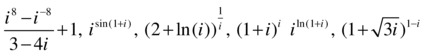
>> (i^8-i^(-8))/(3-4*i) + 1
ans =
1
>> i^(sin(1+i))
ans =
-0.16665202215166 + 0.32904139450307i
>> (2+log(i))^(1/i)
ans =
1.15809185259777 - 1.56388053989023i
>> (1+i)^i
ans =
0.42882900629437 + 0.15487175246425i
>> i^(log(1+i))
ans =
0.24911518828716 + 0.15081974484717i
>> (1+sqrt(3)*i)^(1-i)
ans =
5.34581479196611 + 1.97594883452873i
EXERCISE 3-3
Find the real part, imaginary part, modulus and argument of each of the following:
![]()
>> Z1=i^3*i; Z2=(1+sqrt(3)*i)^(1-i); Z3=(i^i)^i;Z4=i^i;
>> format short
>> real([Z1 Z2 Z3 Z4])
ans =
1.0000 5.3458 0.0000 0.2079
>> imag([Z1 Z2 Z3 Z4])
ans =
0 1.9759 -1.0000 0
>> abs([Z1 Z2 Z3 Z4])
ans =
1.0000 5.6993 1.0000 0.2079
>> angle([Z1 Z2 Z3 Z4])
ans =
0 0.3541 -1.5708 0
EXERCISE 3-4
Consider the matrix M defined as the product of the imaginary unit i with the square matrix of order 3 whose elements are, row by row, the first nine positive integers.
Find the square of M, its square root and its exponential to base 2 and -2.
Find the element-wise Naperian logarithm of M and its element-wise base e exponential.
Find log(M ) and eM.
>> M=i*[1 2 3;4 5 6;7 8 9]
M =
0 + 1.0000i 0 + 2.0000i 0 + 3.0000i
0 + 4.0000i 0 + 5.0000i 0 + 6.0000i
0 + 7.0000i 0 + 8.0000i 0 + 9.0000i
>> C=M^2
C =
-30 -36 -42
-66 -81 -96
-102 -126 -150
>> D=M^(1/2)
D =
0.8570 - 0.2210i 0.5370 + 0.2445i 0.2169 + 0.7101i
0.7797 + 0.6607i 0.9011 + 0.8688i 1.0224 + 1.0769i
0.7024 + 1.5424i 1.2651 + 1.4930i 1.8279 + 1.4437i
>> 2^M
ans =
0.7020 - 0.6146i -0.1693 - 0.2723i -0.0407 + 0.0699i
-0.2320 - 0.3055i 0.7366 - 0.3220i -0.2947 - 0.3386i
-0.1661 + 0.0036i -0.3574 - 0.3717i 0.4513 - 0.7471i
>> (-2)^M
ans =
17.3946 -16.8443i 4.3404 - 4.5696i -7.7139 + 7.7050i
1.5685 - 1.8595i 1.1826 - 0.5045i -1.2033 + 0.8506i
-13.2575 + 13.1252i -3.9751 + 3.5607i 6.3073 - 6.0038i
>> log(M)
ans =
0 + 1.5708i 0.6931 + 1.5708i 1.0986 + 1.5708i
1.3863 + 1.5708i 1.6094 + 1.5708i 1.7918 + 1.5708i
1.9459 + 1.5708i 2.0794 + 1.5708i 2.1972 + 1.5708i
>> exp(M)
ans =
0.5403 + 0.8415i -0.4161 + 0.9093i -0.9900 + 0.1411i
-0.6536 - 0.7568i 0.2837 - 0.9589i 0.9602 - 0.2794i
0.7539 + 0.6570i -0.1455 + 0.9894i -0.9111 + 0.4121i
>> logm(M)
ans =
-5.4033 - 0.8472i 11.9931 - 0.3109i -5.3770 + 0.8846i
12.3029 + 0.0537i -22.3087 + 0.8953i 12.6127 + 0.4183i
-4.7574 + 1.6138i 12.9225 + 0.7828i -4.1641 + 0.6112i
>> expm(M)
ans =
0.3802 - 0.6928i -0.3738 - 0.2306i -0.1278 + 0.2316i
-0.5312 - 0.1724i 0.3901 - 0.1434i -0.6886 - 0.1143i
-0.4426 + 0.3479i -0.8460 - 0.0561i -0.2493 - 0.4602i
EXERCISE 3-5
Consider the vector sum V of the complex vector Z = (i,-i, i) and the real vector R = (0,1,1). Find the mean, median, standard deviation, variance, sum, product, maximum and minimum of the elements of V, as well as its gradient, its discrete Fourier transform and its inverse.
>> Z=[i,-i,i]
Z =
0 + 1.0000i 0 - 1.0000i 0 + 1.0000i
>> R=[0,1,1]
R =
0 1 1
>> V=Z+R
V =
0 + 1.0000i 1.0000 - 1.0000i 1.0000 + 1.0000i
>> [mean(V),median(V),std(V),var(V),sum(V),prod(V),max(V),min(V)]'
ans =
0.6667 - 0.3333i
1.0000 + 1.0000i
1.2910
1.6667
2.0000 - 1.0000i
0 - 2.0000i
1.0000 + 1.0000i
0 - 1.0000i
>> gradient(V)
ans =
1.0000 - 2.0000i 0.5000 0 + 2.0000i
>> fft(V)
ans =
2.0000 + 1.0000i -2.7321 + 1.0000i 0.7321 + 1.0000i
>> ifft(V)
ans =
0.6667 + 0.3333i 0.2440 + 0.3333i -0.9107 + 0.3333i
EXERCISE 3-6
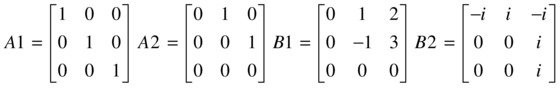
First calculate A = A1 + A2, B = B1 - B2 and C = C1 + C2.
Then calculate AB - BA, A2 + B2 + C2, ABC, sqrt(A) + sqrt B) - sqrt(C), (eB+ eC), their transposes and their inverses.
Finally, check that the product of each of the matrices A, B and C with their inverses gives the identity matrix.
>> A1=eye(3)
A1 =
1 0 0
0 1 0
0 0 1
>> A2=[0 1 0;0 0 1;0 0 0]
A2 =
0 1 0
0 0 1
0 0 0
>> A= A1+A2
A =
1 1 0
0 1 1
0 0 1
>> B1=[0 1 2;0 -1 3;0 0 0]
B1 =
0 1 2
0 -1 3
0 0 0
>> B2=[-i i -i;0 0 i;0 0 i]
B2 =
0 - 1.0000i 0 + 1.0000i 0 - 1.0000i
0 0 0 + 1.0000i
0 0 0 + 1.0000i
>> B=B1-B2
B =
0 + 1.0000i 1.0000 - 1.0000i 2.0000 + 1.0000i
0 -1.0000 3.0000 - 1.0000i
0 0 0 - 1.0000i
>> C1=[1,-1,0;-1,sqrt(2)*i,-sqrt(2)*i;0,0,-1]
C1 =
1.0000 -1.0000 0
-1.0000 0 + 1.4142i 0 - 1.4142i
0 0 -1.0000
>> C2=[0 2 1;1 0 0;1 -1 0]
C2 =
0 2 1
1 0 0
1 -1 0
>> C=C1+C2
C =
1.0000 1.0000 1.0000
0 0 + 1.4142i 0 - 1.4142i
1.0000 -1.0000 -1.0000
>> M1=A*B-B*A
M1 =
0 -1.0000 - 1.0000i 2.0000
0 0 1.0000 - 1.0000i
0 0 0
>> M2=A^2+B^2+C^2
M2 =
2.0000 2.0000 + 3.4142i 3.0000 - 5.4142i
0 - 1.4142i -0.0000 + 1.4142i 0.0000 - 0.5858i
0 2.0000 - 1.4142i 2.0000 + 1.4142i
>> M3=A*B*C
M3 =
5.0000 + 1.0000i -3.5858 + 1.0000i -6.4142 + 1.0000i
3.0000 - 2.0000i -3.0000 + 0.5858i -3.0000 + 3.4142i
0 - 1.0000i 0 + 1.0000i 0 + 1.0000i
>> M4=sqrtm(A)+sqrtm(B)-sqrtm(C)
M4 =
0.6356 + 0.8361i -0.3250 - 0.8204i 3.0734 + 1.2896i
0.1582 - 0.1521i 0.0896 + 0.5702i 3.3029 - 1.8025i
-0.3740 - 0.2654i 0.7472 + 0.3370i 1.2255 + 0.1048i
>> M5=expm(A)*(expm(B)+expm(C))
M5 =
14.1906 - 0.0822i 5.4400 + 4.2724i 17.9169 - 9.5842i
4.5854 - 1.4972i 0.6830 + 2.1575i 8.5597 - 7.6573i
3.5528 + 0.3560i 0.1008 - 0.7488i 3.2433 - 1.8406i
>> inv(A)
ans =
1 -1 1
0 1 -1
0 0 1
>> inv(B)
ans =
0 - 1.0000i -1.0000 - 1.0000i -4.0000 + 3.0000i
0 -1.0000 1.0000 + 3.0000i
0 0 0 + 1.0000i
>> inv(C)
ans =
0.5000 0 0.5000
0.2500 0 - 0.3536i -0.2500
0.2500 0 + 0.3536i -0.2500
>> [A*inv(A) B*inv(B) C*inv(C)]
ans =
1 0 0 1 0 0 1 0 0
0 1 0 0 1 0 0 1 0
0 0 1 0 0 1 0 0 1
>> A'
ans =
1 0 0
1 1 0
0 1 1
>> B'
ans =
0 - 1.0000i 0 0
1.0000 + 1.0000i -1.0000 0
2.0000 - 1.0000i 3.0000 + 1.0000i 0 + 1.0000i
>> C'
ans =
1.0000 0 1.0000
1.0000 0 - 1.4142i -1.0000
1.0000 0 + 1.4142i -1.0000
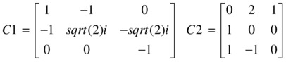
EXERCISE 3-7
Given the matrices
apply the sine function, the base e exponential and logarithm, the square root, the modulus, the argument and the rounding functions.
Calculate eB and ln(A).
>> A=[1 2 3; 4 5 6; 7 8 9]
A =
1 2 3
4 5 6
7 8 9
>> sin(A)
ans =
0.8415 0.9093 0.1411
-0.7568 -0.9589 -0.2794
0.6570 0.9894 0.4121
>> B=[1+i 2+i;3+i,4+i]
B =
1.0000 + 1.0000i 2.0000 + 1.0000i
3.0000 + 1.0000i 4.0000 + 1.0000i
>> sin(B)
ans =
1.2985 + 0.6350i 1.4031 - 0.4891i
0.2178 - 1.1634i -1.1678 - 0.7682i
>> exp(A)
ans =
1.0e+003 *
0.0027 0.0074 0.0201
0.0546 0.1484 0.4034
1.0966 2.9810 8.1031
>> exp(B)
ans =
1.4687 + 2.2874i 3.9923 + 6.2177i
10.8523 + 16.9014i 29.4995 + 45.9428i
>> log(B)
ans =
0.3466 + 0.7854i 0.8047 + 0.4636i
1.1513 + 0.3218i 1.4166 + 0.2450i
>> sqrt(B)
ans =
1.0987 + 0.4551i 1.4553 + 0.3436i
1.7553 + 0.2848i 2.0153 + 0.2481i
>> abs(B)
ans =
1.4142 2.2361
3.1623 4.1231
>> imag(B)
ans =
1 1
1 1
>> fix(sin(B))
ans =
1.0000 1.0000
0 - 1.0000i - 1.0000
>> ceil(log(A))
ans =
0 1 2
2 2 2
2 3 3
>> sign(B)
ans =
0.7071 + 0.7071i 0.8944 + 0.4472i
0.9487 + 0.3162i 0.9701 + 0.2425i
The exponential, square root and logarithm functions used above apply element-wise to the matrix, and have nothing to do with the matrix exponential and logarithmic functions that are used below.
>> expm(B)
ans =
1.0e+002 *
-0.3071 + 0.4625i -0.3583 + 0.6939i
-0.3629 + 1.0431i -0.3207 + 1.5102i
>> logm(A)
ans =
-5.6588 + 2.7896i 12.5041 - 0.4325i -5.6325 - 0.5129i
12.8139 - 0.7970i -23.3307 + 2.1623i 13.1237 - 1.1616i
-5.0129 - 1.2421i 13.4334 - 1.5262i -4.4196 + 1.3313i
EXERCISE 3-8
Solve the following equation in the complex field:
sin(z) = 2
>> vpa(solve('sin(z) = 2'))
ans =
1.316957896924816708625046347308 * i + 1.5707963267948966192313216916398
1.5707963267948966192313216916398 - 1.316957896924816708625046347308 * i
EXERCISE 3-9
Solve the following equations:
a. 1+x+x2+x3+x4+x5 = 0
b. x2 +(6-i)x+8-4i = 0
c. tan(Z) = 3i/5
>> solve('1+x+x^2+x^3+x^4+x^5 = 0')
ans =
-1
-1/2 - (3-^(1/2) * i) / 2
1/2 - (3-^(1/2) * i) / 2
-1/2 + (3 ^(1/2) * i) / 2
1/2 + (3 ^(1/2) * i) / 2
>> solve ('x ^ 2 +(6-i) * x + 8-4 * i = 0')
ans =
-4
i 2
>> vpa (solve ('tan (Z) = 3 * i/5 '))
ans =
0.69314718055994530941723212145818 * i
EXERCISE 3-10
Find the following:
a. The fourth roots of -1 and 1;
b. The fifth roots of 2 + 2i and -1 + i√3;
c. The real part of tan(iLn((a+ib)/(a-ib)));
d. The imaginary part of Z = (2 + i)cos(4-i).
>> solve('x^4+1=0')
ans =
2^(1/2) * (-i/2 - 1/2)
2^(1/2) * (i/2 - 1/2)
2^(1/2) * (1/2 - i/2)
2^(1/2) * (i/2 + 1/2)
>> pretty(solve('x^4+1=0'))
+- -+
| 1/2 / i 1 |
| 2 | - - - - | |
| 2 2 / |
| |
| 1/2 / i 1 |
| 2 | - - - | |
| 2 2 / |
| |
| 1/2 / 1 i |
| 2 | - - - | |
| 2 2 / |
| |
| 1/2 / i 1 |
| 2 | - + - | |
| 2 2 / |
+- -+
>> solve('x^4-1=0')
ans =
-1
1
-i
i
>> vpa(solve('x^5-2-2*i=0'))
ans =
0.19259341768888084906125263406469 * i + 1.2159869826496146992458377919696
-0.87055056329612413913627001747975 * i - 0.87055056329612413913627001747975
0.55892786746600970394985946846702 * i - 1.0969577045083811131206798770216
0.55892786746600970394985946846702 - 1.0969577045083811131206798770216 * i
1.2159869826496146992458377919696 * i + 0.19259341768888084906125263406469
>> vpa(solve('x^5+1-sqrt(3)*i=0'))
ans =
0.46721771281818786757419290603946 * i + 1.0493881644090691705137652947201
1.1424056652180689506550734259384 * i - 0.1200716738059215411240904754285
0.76862922680258900220179378744147 - 0.85364923855044142809268986292246 * i
-0.99480195671282768870147766609475 * i - 0.57434917749851750339931347338896
0.23882781722701229856490119703938 * i - 1.1235965399072191281921551333441
>> simplify(vpa(real(tan(i * log((a+i*b)/(a-i*b))))))
ans =
-0.5 * tanh(conj(log((a^2 + 2.0*a*b*i-1.0*b^2)/(a^2 + b^2))) * i + (0.5 * ((a^2 + 2.0*a*b*i-1.0*b^2)^2 /(a^2 + b^2)^2 - 1) * i) / ((a^2 + 2.0*a*b*i-1.0*b^2)^2 /(a^2 + b^2)^2 + 1))
>> simplify(vpa(imag((2+i)^cos(4-i))))
ans =
-0.62107490808037524310236676683417