![]()
Limits of Sequences and Functions. Continuity in One and Several Variables
Limits
MATLAB incorporates features that allow you to work with limits of sequences and functions. In addition to calculating limits of sequences and functions, one can use these commands to analyze the continuity and differentiability of functions, as well as the convergence of numerical series and power series. The following table summarizes the most common MATLAB functions relating to limits.
|
limit (sequence, inf) |
Calculates the limit of the sequence, indicated by its general term, as n tends to infinity >> syms n ans = 16 /81 |
|
limit(function, x, a) |
Calculates the limit of the function of the variable x, as the variable x tends towards the value a >> syms x ans = 2 |
|
limit(function, a) |
Calculates the limit of the function of the variable x, as the variable x tends towards the value a >> limit((x-1)/(x^(1/2)-1),1) ans = 2 |
|
limit (function, x, a, ‘right’) |
Calculates the limit of the function of the variable x, indicated by its analytical expression, as the variable x tends to a from the right >> syms x ans = Inf |
|
limit (function, x, a, ‘left’) |
Calculates the limit of the function of the variable x, indicated by its analytical expression, as the variable x tends to a from the left >> limit((exp(1/x)),x,0,'left') ans = 0 |
As a first example, we calculate the following sequential limits:
>> syms n

>> limit(((n+3)/(n-1))^n, inf)

ans =

exp(4)

>> limit((1-2/(n+3))^n, inf)

ans =

1/exp(2)

>> limit((1/n)^(1/n), inf)

ans =
1

>> limit(((n+1)^(1/3)-n^(1/3))/((n+1)^(1/2)-n^(1/2)),inf)

ans =

0

>> limit((n^n*exp(-n)*sqrt(2*pi*n))/n^n, n,inf)

ans =

0
In the last limit we have used Sterling’s formula to approximate the factorial.
![]()
As a second example, we calculate the following functional limits:
>> limit(abs(x)/sin(x),x,0)

ans =

NaN

>> syms x
>> limit(abs(x)/sin(x),x,0)

ans =

NaN

>> limit(abs(x)/sin(x),x,0,'left')

ans =

-1

>> limit(abs(x)/sin(x),x,0,'right')

ans =

1

>> limit(abs(x^2-x-7),x,3)

ans =

1
>> limit((x-1)/(x^n-1),x,1)

ans =

1/n

>> limit(exp(1)^(1/x),x,0)

ans =

NaN

>> limit(exp(1)^(1/x),x,0,'left')

ans =

0

>> limit(exp(1)^(1/x),x,0,'right')

ans =

Inf
Sequences of Functions
You can also use the MATLAB commands for limits of sequences and functions described in the preceding table to study the convergence of sequences of functions.
As a first example, consider the sequence of functions defined by gn(x) = (x2+nx) /n with x∈R.
A sensible first approach is to graph the sequence of functions to get an idea of what the limit function might be. To graph these functions we can use both the command plot and the command fplot.
If we use the command fplot, the syntax for the simultaneous graphical representation of the first nine functions of the sequence on the same axes would be as follows:
>> fplot('[(x^2+x),(x^2+2*x)/2,(x^2+3*x)/3,(x^2+4*x)/4,(x^2+5*x)/5,(x^2+5*x)/5,(x^2+6*x)/6,(x^2+7*x)/7,(x^2+8*x)/8,(x^2+9*x)/9]',[-2,2,-2,2])
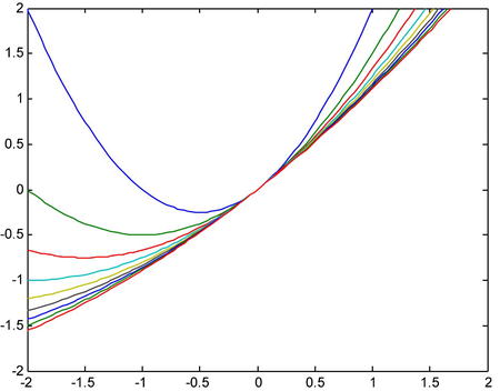
Graphically this indicates that the sequence of functions converges to the identity function f(x) = x.
We can corroborate this fact by using the command limit with the following syntax:
>> syms x n
>> limit((x^2+n*x)/n,n,inf)

ans =

x
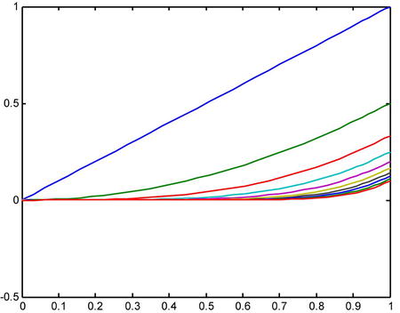
As a second example, we consider the sequence of functions gn(x) = (xn) /n with x∈[0,1].
>> limit(x.^n/n,n,inf);x(1)

ans =

0
Below is the graphical representation of the sequence of functions, which verifies the result.
>> fplot('[x,x^2/2,x^3/3,x^4/4,x^5/5,x^6/6,x^7/7,x^8/8,x^9/9,x^10/10]',
[0,1,-1/2,1])
Continuity
The calculation of limits is a necessary tool when dealing with the concept of continuity. Formally, a function f is continuous at the point x = a if we have:
![]()
If this is not the case, we say the function is discontinuous at a. Thus, for a function f to be continuous at x = a, f must be defined at a, and its value at a must be equal to the limit of f at the point a. If the limit of f(x) as x→ a exists, but is different from f (a) (or f (a) is not defined), then f is discontinuous at a, and f is said to have an avoidable discontinuity at a. The discontinuity can be avoided by appropriately redefining the function at a.
If the two lateral limits of f at a (finite or infinite) exist, but are different, then the discontinuity of f at a is said to be of the “first kind”. The difference between the values of two different lateral limits is called “the jump”. If the difference is finite, the discontinuity is said to be “of the first kind with finite jump” If the difference is infinite, that discontinuity is said to be “of the first kind with infinite jump”. If at least one of the lateral limits does not exist, the discontinuity is said to be “of the second kind”.
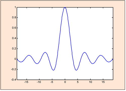
As a first example, we consider the continuity in R-{0} of the function f(x) = sin(x) /x. We will check that. ![]() .
.
>> syms x a
>> limit (sin (x) / x, x, a)

ans =

sin(a) /a
A problem arises at the point x = 0, at which the function f is not defined. Therefore, the function is discontinuous at x = 0. This discontinuity can be avoided by defining the function at x = 0 to have a value equal to ![]() .
.
>> limit (sin(x) / x, x, 0)

ans =

1
Therefore, the function f (x) = sin (x) /x presents an avoidable discontinuity at x = 0 that is avoided by defining f(0) = 1. At all other points the function is continuous. The graph of the function corroborates these findings.
>> fplot ('sin (x) / x', [- 6 * pi, 6 * pi])
As a second example, we observe that the function ![]() is not continuous at the point x = 0 since the lateral boundaries do not match (one is zero and the other infinite).
is not continuous at the point x = 0 since the lateral boundaries do not match (one is zero and the other infinite).
>> syms x

>> limit((exp(1/x)),x,0,'right')

ans =

inf

>> limit((exp(1/x)),x,0, 'left')

ans =

0
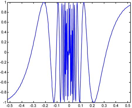
As a third example, we examine the continuity of the function f (x) = sin (1/x). The function f is continuous at any non-zero point, since ![]() :
:
>> syms x a

>> limit(sin(1/x),x,a)

ans =

sin(1/a)
We now consider the point x = 0, at which the function f is not defined. Therefore, the function is discontinuous at x = 0. To try to avoid the discontinuity, we calculate:
>> limit(sin(1/x),x,0)

ans =

limit(sin(1/x), x = 0)

>> limit(sin(1/x),x,0,'left')

ans =

NaN

>> limit(sin(1/x),x,0,'right')

ans =

NaN
We see that at x = 0, the function has a discontinuity of the second kind. The graphical representation confirms this result.
>> fplot('sin(1/x)',[-pi/6,pi/6])
Limits in Several Variables. Iterated and Directional Limits
The generalization of the concept of limit to several variables is quite simple. A sequence of m-dimensional points {(a1n,a2n,...,amn)}, with n running through the natural numbers, has as limit the m-dimensional point (a1,..., am ) if, and only if:
Limit[{a1n}] = a1, Limit[{a2n}] = a2, ..., Limit[{amn}] = am
n→∞                n→∞                    n→∞
This characterization theorem allows us to calculate limits of sequences of m-dimensional points.
There is another theorem similar to the above for the characterization of limits of functions between spaces of more than one dimension. This theorem is used to enable the calculation of limits of multivariable functions.
If f:Rn -> Rm is a function whose m components are (f1 ,f2,...,fm). Then it follows that:
Limit (f1(x1,x2,..,xm),f2(x1,x2,..,xm),...,fn(x1,x2,..,xm)) = (l1,l2,..,ln)  as
x1→a1, x2→a2,..., xm→am

if and only if

Limit (f1(x1,x2,...,xm)) = l1, Limit(f2(x1,x2,...,xm)) = l2,..., Limit(fn(x1,x2,...,xm)) = ln as
x1→a1,...,xm→am
As a first example, we calculate the following three-dimensional limit:
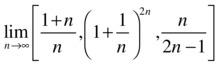
>> syms n
>> V=[limit((n+1)/n,inf),limit((1+1/n)^(2*n),inf),limit(n/(2*n-1),inf)]

V =

[1, exp(2), 1/2]
As a second example, we calculate the following limit:
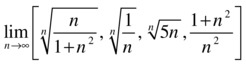
>> syms n
>> V1=[limit((n/(n^2+1))^(1/n),inf),limit((1/n)^(1/n),inf),
       limit((5*n)^(1/n),inf),limit((n^2+1)/n^2,inf)]

V1 =

[1, 1, 1, 1]
As a third example, we calculate ![]() for the function f:R → R2 defined by:
for the function f:R → R2 defined by:
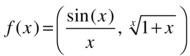
>> syms x
>> V3=[limit(sin(x)/x,x,0),limit((1+x)^(1/x),x,0)]

V3 =

[1, exp(1)]
As fourth example, we find ![]() for the function f:R → R2 defined by:
for the function f:R → R2 defined by:
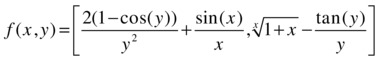
>> [limit(limit(sin(x)/x+2*(1-cos(y))/y^2,x,0),y,0),
   [limit(limit(((1+x)^(1/x)-tan(y)/y),x,0),y,0)]

ans =

[2, exp(1) - 1]
Given a function f: Rn →R an iterated limit of f(x1 ,x2,...,xn) at the point (a1,a2 ,...,an ) is the value of the following limit, if it exists:
Lim    (Lim   (...   (Lim   f(x1,x2,..,xn))...))
x1→a1   x2→a2         xn→an
or any of the other permutations of the limits on xi with i = 1, 2,...,n.
The directional limit of f at the point (a1,..., an), depending on the direction of the curve h(t) =(h1(t) , h2(t),..., hn(t)), such that h(t0) =(a1,a2,...,an), is the value:
Lim (f(h(t))) = Lim f(x1,x2,...,xn)
t→t0              (x1,x2,...,xn)→(a1, a2,...,an)
A necessary condition for a function of several variables to have a limit at a point is that all the iterated limits have the same value (which will be equal to the value of the limit of the function, if it exists). The directional limits of a function at a point may be different for different curves, and some of the directional limits may not exist. Another necessary condition for a function of several variables to have a limit at a point is that all directional limits, approaching along any curve, have the same value (and this common value will be equal to the value of the limit of the function, if it exists). Therefore, to prove that a function has no limit it is enough to show that the iterated limits do not exist, or if they exist, are not the same, or that two directional limits are different, or a directional limit doesn’t exist. Another practical procedure to calculate the limit of a function of several variables is to change the coordinates from Cartesian to polar, which can facilitate the limit operation.
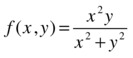
As first example, we calculate ![]() for f: R2 → R defined by:
for f: R2 → R defined by:
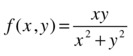
>> syms x y
>> limit(limit((x*y)/(x^2+y^2),x,0),y,0)

ans =

0

>> limit(limit((x*y)/(x^2+y^2),y,0),x,0)

ans =

0
We see that the iterated limits are the same. Next we calculate the directional limits according to the family of straight lines y = mx:
>> syms m
>> limit((m*x^2)/(x^2+(m^2)*(x^2)),x,0)

ans =

m/(1+m^2)
We see that the directional limits depend on the parameter m, which will be different for different values of m (for the different considered straight lines). Thus, we conclude that the function has no limit at (0,0).
The result can be graphically illustrated as a surface as follows.
>> ezsurf('(x*y) /(x^2+y^2)')
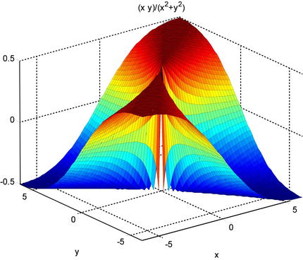
We observe that in a neighborhood of (0,0), the function has no limit.
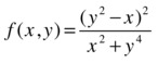
As second example, we consider ![]() for the function f:R2 → R defined by:
for the function f:R2 → R defined by:
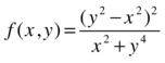
>> syms x y
>> limit(limit((y^2-x^2)^2/(y^4+x^2),x,0),y,0)

ans =

1

>> limit(limit((y^2-x^2)^2/(y^4+x^2),y,0),x,0)

ans =

0
As the iterated limits are different, we conclude that the function has no limit at the point (0,0).
If we graph the surface in a neighborhood of (0,0) we can observe its behavior at that point.
>> ezsurf('(y^2-x^2)^2/(y^4+x^2)',[-1 1], [-1 1])
Continuity in Several Variables
Generalizing the definition of continuity in one variable we can easily formalize the concept of continuity in several variables. A function f: Rn →Rm is said to be continuous at the point (a1,a2,..., an) if:
Lim f(x1,x2,...,xn) = f(a1,a2,...,an)
x1→a1, x2→a2,..., xn→an
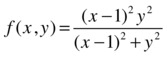
As a first example, we examine the continuity at the point (1,2) of the function:
![]() if
if ![]() and
and ![]() .
.
>> limit(limit((x^2+2*y),x,1),y,2)

ans =

5

>> limit(limit((x^2+2*y),y,2),x,1)

ans =

5
We see that if the limit at (1,2) exists, then it should be 5. But the function has value 0 at the point (1,2). Thus, the function is not continuous at the point (1,2).
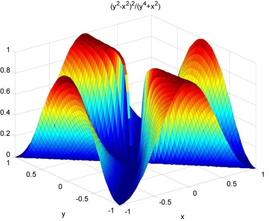
As a second example, we study the continuity in all of R2 of the function ![]() .
.
>> syms x y a b
>> limit(limit((x^2+2*y),x,a),y,b)

ans =

a^2 + 2*b

>> limit(limit((x^2+2*y),y,b),x,a)

ans =

a^2 + 2*b

>> f='x^2+2*y'

f =

x^2+2*y

>> subs(f,{x,y},{a,b})

ans =

a^2 + 2*b
We see that the iterated limits coincide and their common value coincides with the value of the function at the generic point (a, b) in R2, i.e. ![]() .
.
If we graphically represent the surface, we see that the function is continuous across its domain of definition.
>> ezsurf('x^2+2*y')
EXERCISE 5-1
Calculate the following limits:
The first limit presents a typical uncertainty of the type ![]() :
:
>> limit((3*n^3+7*n^2+1)/(4*n^3-8*n+5),n,inf)
ans =
3/4
The last two limits are of the type ![]() and
and ![]() :
:
>> limit(((n+1)/2)*((n^4+1)/n^5), inf)
ans =
1/2
>> limit(((n+1)/n^2)^(1/n), inf)
ans =
1
EXERCISE 5-2
Calculate the following limits:
Here we have three indeterminates of the type 0/0 and one of the form ![]() :
:
>> syms x
>> limit((x-(x+2)^(1/2))/((4*x+1)^(1/2)-3),2)
ans =
9/8
>> limit((1+x)^(1/x))
ans =
exp(1)
>> syms x a, limit(sin(a*x)^2/x^2,x,0)
ans =
a^2
>> limit((exp(1)^x-1)/log(1+x))
ans =
log(3060513257434037/1125899906842624)
>> vpa(limit((exp(1)^x-1)/log(1+x)))
ans =
1.0000000000000001101889132838495
EXERCISE 5-3
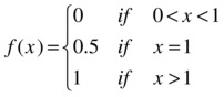
Calculate the limit of the following sequence of functions:
 x > 0
x > 0
We will start by graphically representing the functions to predict the possible limit.
>> fplot('[x/(1+x),x^2/(1+x^2),x^3/(1+x^3),x^4/(1+x^4),x^5/(1+x^5), x^6/(1+x^6),x^7/(1+x^7),x^8/(1+x^8),x^9/(1+x^9),x^10/(1+x^10)]',[0,1,-1/2,1])
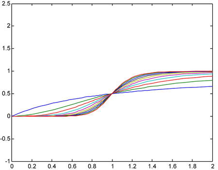
This tells us that, intuitively, the limit is the x-axis (i.e. the function f (x) = 0) for values of x in [0,1], the value 0.5 for x = 1 and the function f (x) = 1 for x > 1. Let’s see:
>> vpa(simplify(limit(x^n/(1+x^n),n,inf)))
ans =
piecewise([x = 1.0, 0.5], [1.0 < x, 1.0], [x < 1.0, 0.0])
MATLAB tells us that the limit function is:
EXERCISE 5-4
Find ![]() for the function f:R2 → R defined by:
for the function f:R2 → R defined by:
>> syms x y m, limit(limit((y^2-x)^2/(y^4+x^2),y,0),x,0)
ans =
1
>> limit(limit((y^2-x)^2/(y^4+x^2),x,0),y,0)
ans =
1
We see that the iterated limits are the same. We then calculate the directional limits according to the family of straight lines y = mx:
>> limit(((m*x)^2-x)^2/((m*x)^4+x^2),x,0)
ans =
1
The directional limits according to the family of straight lines y = mx do not depend on m and coincide with the iterated limits. We now find the directional limits according to the family of parabolas y ^ 2 = mx:
>> limit(((m*x)-x)^2/((m*x)^2+x^2),x,0)
ans =
(m - 1)^2/(m^2 + 1)
The directional limits according to this family of parabolas depend on the parameter, and so they are different. This leads us to conclude that the function has no limit at (0,0).
EXERCISE 5-5
Find ![]() for the function f:R2 → R defined by:
for the function f:R2 → R defined by:
>> syms x y, limit(limit((x^2*y)/(x^2+y^2),x,0),y,0)
ans =
0
>> limit(limit((x^2*y)/(x^2+y^2),x,0),y,0)
ans =
0
>> limit(((x^2)*(m*x))/(x^2+(m*x)^2),x,0)
ans =
0
>> limit(((m*y)^2)*y/((m*y)^2+y^2),y,0)
ans =
0
We see that the iterated limits and the directional limits according to the given families of lines and parabolas all coincide and are equal to zero. This leads us to suspect that the limit of the function may be zero. To confirm this, we transform to polar coordinates and find the limit:
>> syms a r;
>> limit(limit(((r^2) * (cos(a)^2) * (r) * (sin(a))) / ((r^2) * (cos(a) ^ 2) +(r^2) * (sin(a)^2)), r, 0), a, 0)
ans =
0
We therefore conclude that the limit of the function is zero at the point (0,0).
This is an example where as a last resort we had to transform to polar coordinates. We used families of lines and parabolas for our directional limits, but other curves could have been used. A change to polar coordinates can be crucial in determining the limits of functions of several variables. As we have seen, there are sufficient criteria for a function to have no limit at a point, but there are no necessary and sufficient conditions to ensure the existence of a limit.
EXERCISE 5-6
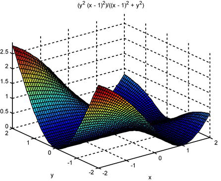
Find ![]() for f: R2 → R defined by:
for f: R2 → R defined by:
>> syms x y m a r
>> limit (limit (y ^ 2 *(x-1) ^ 2 / (y ^ 2 +(x-1) ^ 2), x, 0), y, 0)
ans =
0
>> limit (limit (y ^ 2 *(x-1) ^ 2 / (y ^ 2 +(x-1) ^ 2), y, 0), x, 0)
ans =
0
>> limit ((m*x) ^ 2 *(x-1) ^ 2/((m*x) ^ 2 +(x-1) ^ 2), x, 0)
ans =
0
>> limit ((m*x) *(x-1) ^ 2/((m*x) +(x-1) ^ 2), x, 0)
ans =
0
We see that the iterated and directional limits coincide. Next we calculate the limit in polar coordinates:
>> limit(limit((r ^ 2 * sin(a) ^ 2) * (r * cos(a) - 1) ^ 2 / ((r ^ 2 * sin(a) ^ 2) + (r * cos(a) - 1) ^ 2), r, 1), a, 0)
ans =
0
The limit is zero at the point (1,0). Below we graph the surface, observing the tendency to 0 in a neighborhood of (1,0):
>> ezsurf (y ^ 2 *(x-1) ^ 2 / (y ^ 2 +(x-1) ^ 2), [- 2, 2, - 2, 2])
EXERCISE 5-7
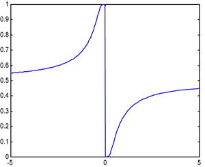
Study the continuity of the function of a real variable:
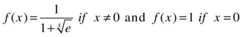
The only problematic point is at x = 0. Now, the function does exist at x = 0 (it has value 1). We will try to find the lateral limits as x→0 :
>> syms x
>> limit(1 /(1 + exp(x)), x, 0, 'right')
ans =
0
>> limit(1/(1 + exp(x)), x, 0, 'left')
Warning: Could not attach the property of being close to the limit to variable limit point
[limit]
ans =
1
As the lateral limits are different, the limit of the function as x→0 does not exist. But as the lateral limits are finite, the discontinuity of the first kind at x = 0 is a finite jump. This is illustrated in Figure 5-1:
>> fplot ('1 /(1 + exp(x))'[-5, 5])