
![]()
Derivatives. One and Several Variables
Derivatives
MATLAB implements a special set of commands enabling you to work with derivatives, which is particularly important in the world of computing and its applications. The derivative of a real function at a point measures the instantaneous rate of change of that function in a neighborhood of the point; i.e. how the dependent variable changes as a result of a small change in the independent variable. Geometrically, the derivative of a function at a point is the slope of the tangent to the function at that point. The origin of the idea derived from the attempt to draw the tangent line at a given point on a given curve.
A function f(x) defined in a neighborhood of a point a is said to be differentiable at a if the following limit exists:
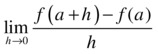
The value of the limit, if it exists, is denoted by f'(a), and is called the derivative of the function f at the point a. If f is differentiable at all points of its domain, it is simply said to be differentiable. The continuity of a function is a necessary (but not sufficient) condition for differentiability, and any differentiable function is continuous.
The following table shows the basic commands that enable MATLAB to work with derivatives.
|
diff('f', 'x') |
Finds the derivative of f with respect to x >> diff('sin(x^2)','x') ans = 2*x*cos(x^2) |
|
syms x, diff(f,x) |
Finds the derivative of f with respect to x >> syms x ans = 2*x*cos(x^2) |
|
diff('f', 'x', n) |
Finds the nth derivative of f with respect to x >> diff('sin(x^2)','x',2) ans = 2*cos(x^2) - 4*x^2*sin(x^2) |
|
syms x, diff(f, x, n) |
Finds the nth derivative of f with respect to x >> syms x ans = 2*cos(x^2) - 4*x^2*sin(x^2) |
|
R = jacobian(w,v) |
Finds the Jacobian matrix of w with respect to v >> syms x y z ans = [ y*z, x*z, x*y] [ 0, 1, 0] [ 1, 0, 1] |
|
Y = diff(X) |
Calculates differences between adjacent elements of the vector X: [X(2)-X(1), X(3)-X(2), ..., X(n)-X(n-1)]. If X is an m×n matrix, diff(X) returns the row difference matrix: [X(2:m,:)-X(1:m-1,:)] x = [1 2 3 4 5]; y = diff(x) y = 1 1 1 1 |
|
Y = diff(X,n) |
Finds differences of order n, for example: diff(X,2)=diff(diff(X)) x = [1 2 3 4 5]; z = diff(x,2) z = 0 0 0 |
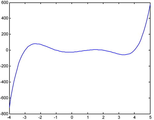
As a first example, we consider the function f(x) = x5-3x4-11x3+27x2+10x-24 and graph its derivative in the interval [-4,5].
>> x=-4:0.1:5;
>> f=x.^5-3*x.^4-11*x.^3+27*x.^2+10*x-24;
>> df=diff(f)./diff(x);
>> plot(x,f)
As a second example, we calculate the derivative of the function log(sin(2x)) and simplify the result.
>> pretty(simplify(diff('log(sin(2*x))','x')))

  2 cot(2 x)
As a third example, we calculate the first four derivatives of the following function:
f(x) = 1/x2

>> f='1/x^2'

f =
1/x^2

>> [diff(f),diff(f,2),diff(f,3),diff(f,4)]

ans =

[ -2/x^3, 6/x^4, -24/x^5, 120/x^6]
The MATLAB commands for differentiation described above can also be used for partial differentiation.
As an example, given the function f(x,y) = sin(xy)+cos(xy2), we calculate:
∂f/∂x, ∂f/∂y, ∂2f/∂x2, ∂2f/∂y2, ∂2f/∂x∂y, ∂2f/∂y∂x and ∂4f/∂2x∂2y

>> syms x y
>> f=sin(x*y)+cos(x*y^2)

f =

sin(x*y)+cos(x*y^2)

>> diff(f,x)

ans =

cos(x*y)*y-sin(x*y^2)*y^2

>> diff(f,y)

ans =

cos(x*y)*x-2*sin(x*y^2)*x*y

>> diff(diff(f,x),x)

ans =

-sin(x*y)*y^2-cos(x*y^2)*y^4

>> diff(diff(f,y),y)

ans =

-sin(x*y)*x^2-4*cos(x*y^2)*x^2*y^2-2*sin(x*y^2)*x

>> diff(diff(f,x),y)

ans =

-sin(x*y)*x*y+cos(x*y)-2*cos(x*y^2)*x*y^3-2*sin(x*y^2)*y

>> diff(diff(f,y),x)

ans =

-sin(x*y)*x*y+cos(x*y)-2*cos(x*y^2)*x*y^3-2*sin(x*y^2)*y

>> diff(diff(diff(diff(f,x),x),y,y))

ans =

sin(x*y)*y^3*x-3*cos(x*y)*y^2+2*cos(x*y^2)*y^7*x+6*sin(x*y^2)*y^5
Applications of Differentiation. Tangents, Asymptotes, Extreme Points and Points of Inflection
A direct application of differentiation allows us to find the tangent to a function at a given point, horizontal, vertical and oblique asymptotes of a function, intervals of increase and concavity, maxima and minima and points of inflection.
With this information it is possible to give a complete study of curves and their representation.
If f is a function which is differentiable at x0, then f ' (x0) is the slope of the tangent line to the curve y = f(x) at the point (x0, f (x0)). The equation of the tangent will be ![]() .
.
The horizontal asymptotes of the curve ![]() are limit tangents, as
are limit tangents, as ![]() , which are horizontal. They are defined by the equation
, which are horizontal. They are defined by the equation ![]() .
.
The vertical asymptotes of the curve ![]() are limit tangents, as
are limit tangents, as ![]() , which are vertical. They are defined by the equation
, which are vertical. They are defined by the equation ![]() , where x0 is a value such that
, where x0 is a value such that ![]() .
.
The oblique asymptotes to the curve ![]() at the point
at the point ![]() have the equation
have the equation ![]() , where
, where  And
And ![]() .
.
If f is a function for which f ' (x0) and f ' ' (x0) both exist, then, if ![]() and
and ![]() , the function f has a local maximum at the point(x0, f (x0)).
, the function f has a local maximum at the point(x0, f (x0)).
If f is a function for which f ' (x0) and f ' ' (x0) both exist, then, if ![]() and
and ![]() , the function f has a local minimum at the point(x0, f (x0)).
, the function f has a local minimum at the point(x0, f (x0)).
If f is a function for which f ' (x0), f ' ' (x0) and f ' ' ' (x0) exist, then, if ![]() and
and ![]() and f ' ' ' (x0) 0, the function f has a turning point at the point(x0, f(x0)).
and f ' ' ' (x0) 0, the function f has a turning point at the point(x0, f(x0)).
If f is differentiable, then the values of x for which the function f is increasing are those for which f ' (x) is greater than zero.
If f is differentiable, then the values of x for which the function f is decreasing are those for which f ' (x) is less than zero.
If f is twice differentiable, then the values of x for which the function f is concave are those for which f ' ' (x) is greater than zero.
If f is twice differentiable, then the values of x for which the function f is convex are those for which f ' ' (x) is less than zero.
As an example, we perform a comprehensive study of the function:
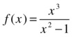
calculating the asymptotes, maxima, minima, inflexion points, intervals of increase and decrease and intervals of concavity and convexity.
>> f='x^3/(x^2-1)'

f =

x^3/(x^2-1)

>> syms x, limit(x^3/(x^2-1),x,inf)

ans =

NaN
Therefore, there are no horizontal asymptotes. To see if there are vertical asymptotes, we consider the values of x that make the function infinite:
>> solve('x^2-1')

ans =

[ 1]
[-1]
The vertical asymptotes are the lines x = 1 and x = -1. Let us see if there are any oblique asymptotes:
>> limit(x^3/(x^2-1)/x,x,inf)

ans =

1

>> limit(x^3/(x^2-1)-x,x,inf)

ans =

0
The line y = x is an oblique asymptote. Now, the maxima and minima, inflection points and intervals of concavity and growth will be analyzed:
>> solve(diff(f))

ans =

[       0]
[       0]
[ 3^(1/2)]
[-3^(1/2)]
The first derivative vanishes at the points with abscissa x = 0, x =√ 3 and x = - √ 3. These points are candidates for maxima and minima. To determine whether they are maxima or minima, we find the value of the second derivative at these points:
>> [numeric(subs(diff(f,2),0)),numeric(subs(diff(f,2),sqrt(3))),
    numeric(subs(diff(f,2),-sqrt(3)))]

ans =

         0    2.5981   -2.5981
Therefore, at the point with abscissa x = - √3 there is a maximum and at the point with abscissa x = √ 3 there is a minimum. At x = 0 we know nothing:
>> [numeric(subs(f,sqrt(3))),numeric(subs(f,-sqrt(3)))]

ans =

    2.5981   -2.5981
Therefore, the maximum point is (- √ 3, -2.5981) and the minimum point is (√ 3, 2.5981).
We will now analyze the inflection points:
>> solve(diff(f,2))

ans =

[         0]
[ i*3^(1/2)]
[-i*3^(1/2)]
The only possible point of inflection occurs at x = 0, and since f (0) = 0, the possible turning point is (0, 0):
>> subs(diff(f,3),0)

ans =

-6
As the third derivative at x = 0 does not vanish, the origin is indeed a turning point:
>> pretty(simple(diff(f)))

                              2   2
                            x  (x  - 3)
                            ------------
                                2     2
                             (x  - 1)
The curve is increasing when y ' > 0, i.e., in the intervals (- ∞, - √ 3) and (√ 3, ∞).
The curve is decreasing when y ' < 0, that is, in the intervals (-√3,-1), (-1,0), (0,1) and (1, √3).
>> pretty(simple(diff(f,2)))

                                   2
                              x (x  + 3)
                           2 ------------
                                  2     3
                               (x  - 1)
The curve will be concave when y'' > 0, that is, in the intervals (-1,0) and (1, ∞).
The curve will be convex when y'' < 0, that is, in the intervals (0,1) and (- ∞, -1).
The curve has horizontal tangents at the three points at which the first derivative is zero. The equations of the horizontal tangents are y = 0, y = 2.5981 and y = -2.5981.
The curve has vertical tangents at the points that make the first derivative infinite. These points are x = 1 and x = -1. Therefore, the vertical tangents coincide with the two vertical asymptotes.
Next, we graph the curve together with its asymptotes:
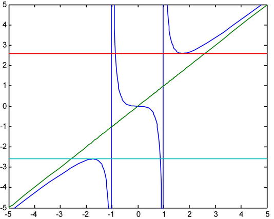
>> fplot('[x^3/(x^2-1),x]',[-5,5,-5,5])
We can also represent the curve, its asymptotes and their horizontal and vertical tangents in the same graph.
>> fplot('[x^3/(x^2-1),x,2.5981,-2.5981]',[-5,5,-5,5])
Differentiation in Several Variables
The concept of differentiation for functions of one variable is generalizable to differentiation for functions of several variables. Below we consider partial derivatives for the case of two variable functions.
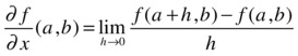
Given the function f: R2 → R, the partial derivative of f with respect to the variable x at the point (a, b) is defined as follows:
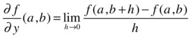
In the same way, the partial derivative of f with respect to the variable y at the point (a, b) is defined in the following way:
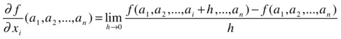
Generally speaking, we can define the partial derivative with respect to any variable for a function of n variables.
Given the function f: Rn → R, the partial derivative of f with respect to the variable xi (i = 1,2,...,n) at the point (a1,a2,...,an) is defined as follows:
The function f is differentiable if all partial derivatives with respect to xi (i = 1,2,...,n) exist and are continuous.
Every differentiable function is continuous, and if a function is not continuous it cannot be differentiable.
The directional derivative of the function f with respect to the vector v=(v1,v2,...,vn) is defined as the following scalar product:
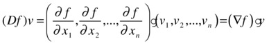
 is called the gradient vector of f.
The directional derivative of the function f with respect to the vector v =(dx1,dx2,...,dxn) is called the total differential of f. Its value is:
Partial derivatives can be calculated using the MATLAB commands for differentiation that we already know.
|
diff(f(x,y,z,...),x) |
Partial derivative of f with respect to x >> syms x y z >> diff(x^2+y^2+z^2+x*y-x*z-y*z+1,z) ans = 2*z - y - x |
|
diff (f(x,y,z,...), x, n) |
Nth partial derivative of f with respect to x >> diff(x^2+y^2+z^2+x*y-x*z-y*z+1,z,2) ans = 2 |
|
diff(f(x1,x2,x3,...),xj) |
Partial derivative of f with respect to xj >> diff(x^2+y^2+z^2+x*y-x*z-y*z+1,y) ans = x + 2*y - z |
|
diff(f(x1,x2,x3,...),xj,n) |
Nth partial derivative of f with respect to xj >> diff(x^2+y^2+z^2+x*y-x*z-y*z+1,y,2) ans = 2 |
|
diff(diff(f(x,y,z,...),x),y)) |
The second partial derivative of f with respect to x and y >> diff(diff(x^2+y^2+z^2+x*y-x*z-y*z+1,x), y) ans = 1 |
As a first example, we study the differentiability and continuity of the function:
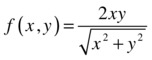 if
if ![]() and
and ![]()
To see if the function is differentiable, it is necessary to check whether it has continuous partial derivatives at every point. We consider any point other than the origin and calculate the partial derivative with respect to the variable x:
>> syms x y
>> pretty(simplify(diff((2*x*y)/(x^2+y^2)^(1/2),x)))

        3
     2 y
  ----------
           3
           -
           2
    2    2
  (x  + y )
Now, let's see if this partial derivative is continuous at the origin. When calculating the iterated limits at the origin, we observe that they do not coincide.
>> limit(limit(2*y^3/(x^2+y^2)^(3/2),x,0),y,0)

ans =

NaN

>> limit(limit(2*y^3/(x^2+y^2)^(3/2),y,0),x,0)

ans =

0
The limit of the partial derivative does not exist at (0, 0), so we conclude that the function is not differentiable.
However, the function is continuous, since the only problematic point is the origin, and the limit of the function is 0 = f (0, 0):
>> limit(limit((2*x*y)/(x^2+y^2)^(1/2),x,0),y,0)

ans =

0

>> limit(limit((2*x*y)/(x^2+y^2)^(1/2),y,0),x,0)

ans =

0

>> m = sym('m', 'positive')
>> limit((2*x*(m*x))/(x^2+(m*x)^2)^(1/2),x,0)

ans =

0

>> a = sym ('a', 'real'),
>> f =(2*x*y) /(x^2+y^2) ^(1/2);
>> limit(subs(f,{x,y},{r*cos(a),r*sin(a)}),r,0)

ans =

0
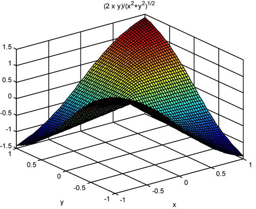
The iterated limits and the directional limits are all zero, and by changing the function to polar coordinates, the limit at the origin turns out to be zero, which coincides with the value of the function at the origin. Thus this is an example of a non-differentiable continuous function. A graphical representation helps us to interpret the result.
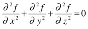
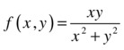
As a second example, we consider the function:
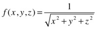
We verify the equation:
>> syms x y z
>> f=1/(x^2+y^2+z^2)^(1/2)

f =

1/(x^2 + y^2 + z^2)^(1/2)

>> diff(f,x,2)+diff(f,y,2)+diff(f,z,2)

ans =

(3*x^2)/(x^2 + y^2 + z^2)^(5/2) - 3/(x^2 + y^2 + z^2)^(3/2) + (3*y^2)/(x^2 + y^2 + z^2)^(5/2) + (3*z^2)/(x^2 + y^2 + z^2)^(5/2)

>> simplify(diff(f,x,2)+diff(f,y,2)+diff(f,z,2))

ans =

0
As a third example, we calculate the directional derivative of the function:

at the point (2,1,1) in the direction of the vector v= (1,1,0). We also find the gradient vector of f.
Recall that the directional derivative of the function f in the direction of the vector v= (v1,v2,...,vn) is defined as the following dot product:

 is called the gradient vector of f.
First, we calculate the gradient of the function f.
>> syms x y z
>> f=1/(x^2+y^2+z^2)^(1/2)

f =

1/(x^2 + y^2 + z^2)^(1/2)

>> Gradient_f=simplify([diff(f,x),diff(f,y),diff(f,z)])

Gradient_f =

[ -x/(x^2 + y^2 + z^2)^(3/2), -y/(x^2 + y^2 + z^2)^(3/2), -z/(x^2 + y^2 + z^2)^(3/2)]
We then calculate the gradient vector at the point (2,1,1).
>> Gradient_f_p = subs(Gradient_f,{x,y,z},{2,1,1})

Gradient_f_p =

   -0.1361   -0.0680   -0.0680
Finally, we calculate the directional derivative.
>> Directional_derivative_p = dot(Gradient_f_p, [1,1,0])

Directional_derivative_p =

-0.2041
Extreme Points in Several Variables
MATLAB allows you to easily calculate maxima and minima of functions of several variables.
A function f: Rn→R, which maps the point (x1, x2,..., xn)ÎR to f(x1,x2,...,xn)ÎR, has an extreme point at (a1, a2, ..., an) if the gradient vector 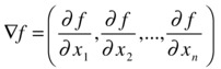 is zero at (a1, a2, ..., an).
By setting all the first order partial derivatives equal to zero and solving the resulting system, we can find the possible maxima and minima.
To determine the nature of the extreme point, it is necessary to construct the Hessian matrix, which is defined as follows:
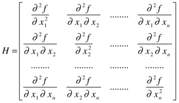
First, suppose that the determinant of H is non-zero at the point(a1, a2, ..., an). In this case, we say that the point is non-degenerate and, in addition, we can determine the nature of the extreme point via the following conditions:
If the Hessian matrix at the point (a1, a2, ..., an) is positive definite, then the function has a minimum at that point.
If the Hessian matrix at the point (a1, a2, ..., an) is negative definite, then the function has a maximum at that point.
In any other case, the function has a saddle point at(a1, a2, ..., an).
If the determinant of H is zero at the point(a1, a2, ..., an), we say that the point is degenerate.
As an example, we find and classify the extreme points of the function:
![]()
We start by finding the possible extreme points. To do so, we set the partial derivatives with respect to all the variables (i.e. the components of the gradient vector of f ) equal to zero and solve the resulting system in three variables:
>> syms x y z
>> f=x^2+y^2+z^2+x*y

f =

x^2 + x*y + y^2 + z^2

>> [x y z] = solve(diff(f,x), diff(f,y), diff(f,z), x, y, z)

x =

0

y =

0

z =

0
The single extreme point is the origin (0,0,0). We will analyze what kind of extreme point it is. To do this, we calculate the Hessian matrix and express it as a function of x, y and z:
>> clear all
>> syms x y z
>> f=x^2+y^2+z^2+x*y

f =

x^2 + x*y + y^2 + z^2

>> diff(f,x)

ans =

2*x + y

>> H=simplify([diff(f,x,2),diff(diff(f,x),y),diff(diff(f,x),z);
               diff(diff(f,y),x),diff(f,y,2),diff(diff(f,y),z);
                    diff(diff(f,z),x),diff(diff(f,z),y),diff(f,z,2)])

H =

[ 2, 1, 0]
[ 1, 2, 0]
[ 0, 0, 2]

>> det(H)

ans =

6
We have seen that the Hessian matrix is constant (i.e. it does not depend on the point at which it is applied), therefore its value at the origin is already found. The determinant is non-zero, so there are no degenerate extreme points.
>> eig(H)

ans =

 1
 2
 3
We see that the Hessian matrix at the origin is positive definite, because its eigenvalues are all positive. We then conclude that the origin is a minimum of the function.
MATLAB additionally incorporates specific commands for the optimization and search for zeros of functions of several variables. The following table shows the most important ones.
|
g = inline(expr) |
Constructs an inline function from the string expr >> g = inline('t^2') g = Inline function: g(t) = t^2 |
|
g = inline(expr,arg1,arg2, ...) |
Constructs an inline function from the string expr with the given input arguments >> g = inline('sin(2*pi*f + theta)', 'f', 'theta') g = Inline function: g(f,theta) = sin(2*pi*f + theta) |
|
g = inline(expr,n) |
Constructs an inline function from the string expr with n input arguments >> g = inline('x^P1', 1) g = Inline function: g(x,P1) = x^P1 |
|
f = @function |
Enables the function to be evaluated >> f = @cos f = @cos >> ezplot(f, [-pi,pi]) |
|
x = fminbnd(fun,x1,x2) |
Returns the minimum of the function in the interval (x1, x2) >> x = fminbnd(@cos,3,4) x = 3.1416 |
|
x = fminbnd(fun,x1,x2,options) |
Returns the minimum of the function in the interval (x1, x2) according to the option given by optimset (...). This last command is explained later. >> x = fminbnd(@cos,3,4,optimset('TolX',1e-12,'Display','off')) x = 3.1416 |
|
x = fminbnd(fun,x1,x2,options,P1,P2,..) |
Specifies additional parameters P1, P2,... to pass to the target function fun(x,P1,P2,...) |
|
[x, fval] = fminbnd (...) |
Returns the value x and the value of the function at x at which the objective function has a minimum >> [x,fval] = fminbnd(@cos,3,4) x = 3.1416 fval = -1.0000 |
|
[x, fval, f] = fminbnd (...) |
In addition returns an indicator of convergence of f (f > 0 indicates convergence to the solution, f < 0 no convergence and f = 0 exceeds the number of steps) >> [x,fval,f] = fminbnd(@cos,3,4) x = 3.1416 fval = -1.0000 f = 1 |
|
[x,fval,f,output] = fminbnd(...) |
Gives further information on optimization (output.algorithm gives the algorithm used, output.funcCount gives the number of evaluations of fun and output.iterations gives the number of iterations) >> [x,fval,f,output] = fminbnd(@cos,3,4) x = 3.1416 fval = -1.0000 f = 1 output = iterations: 7 funcCount: 8 algorithm: 'golden section search, parabolic interpolation' message: [1x112 char] |
|
x = fminsearch(fun,x0) x = fminsearch(fun,x0,options) x = fminsearch(fun,x0,options,P1,P2,...) [x,fval] = fminsearch(...) [x,fval,f] = fminsearch(...) [x,fval,f,output] = fminsearch(...) |
Minimizes a function of several variables with initial values given by x0. The argument x0 can be an interval [a, b] in which a solution is sought. Then, to minimize fun in [a, b], the command x = fminsearch (fun, [a, b]) is used. >> x=fminsearch(inline('(100*(1-x^2)^2+(1-x)^2)'),3) x = 1.0000 >> [x,feval]=fminsearch(inline('(100*(1-x^2)^2 +(1-x)^2)'),3) x = 1.0000 feval = 2.3901e-007 >> [x,feval,f]=fminsearch(inline('(100*(1-x^2)^2 +(1-x)^2)'),3) x = 1.0000 feval = 2.3901e-007 f = 1 >> [x,feval,f,output]=fminsearch(inline('(100*(1-x^2)^2+(1-x)^2)'),3) x = 1.0000 feval = 2.3901e-007 f = 1 output = iterations: 18 funcCount: 36 algorithm: 'Nelder-Mead simplex direct search' message: [1x196 char] |
|
x = fzero x0 (fun) x = fzero(fun,x0,options) x = fzero(fun,x0,options,P1,P2,...) [x, fval] = fzero (...) [x, fval, exitflag] = fzero (...) [x,fval,exitflag,output] = fzero(...) |
Finds zeros of functions. The argument x0 can be an interval [a, b] in which a solution is sought. Then, to find a zero of fun in [a, b] the command x = fzero (fun, [a, b]) is used, where fun has opposite signs at a and b. >> x = fzero(@cos,[1 2]) x = 1.5708 >> [x,feval] = fzero(@cos,[1 2]) x = 1.5708 feval = 6.1232e-017 >> [x,feval,exitflag] = fzero(@cos,[1 2]) x = 1.5708 feval = 6.1232e-017 exitflag = 1 >> [x,feval,exitflag,output] = fzero(@cos,[1 2]) x = 1.5708 feval = 6.1232e-017 exitflag = 1 output = interval iterations: 0 iterations: 5 funcCount: 7 algorithm:'bisection, interpolation'message: 'Zero found in |
|
options = optimset('p1',v1,'p2',v2,...) |
Creates optimization options parameters p1, p2,... with values v1, v2... The possible parameters are Display (with possible values 'off', 'iter', 'final', 'notify' to hide the output, display the output of each iteration, display only the final output and show a message if there is no convergence); MaxFunEvals, whose value is an integer indicating the maximum number of evaluations; MaxIter whose value is an integer indicating the maximum number of iterations; TolFun, whose value is an integer indicating the tolerance in the value of the function, and TolX, whose value is an integer indicating the tolerance in the value of x |
|
Val = optimget (options, 'param') |
Returns the value of the parameter specified in the optimization options structure |
As a first example, we minimize the function cos(x) in the interval (3,4).
>> x = fminbnd(inline('cos(x)'),3,4)

x =

    3.1416
In the following example we conduct the same minimization with a tolerance of 8 decimal places and find both the value of x that minimizes the cosine in the range given and the minimum value of the cosine function in that interval, presenting information relating to all iterations of the process.
>> [x, fval, f] = fminbnd (@cos, 3, 4, optimset('TolX',1e-8,...)) (( 'Display', 'iter'));

 Func-count     x          f(x)         Procedure
    1        3.38197    -0.971249        initial
    2        3.61803    -0.888633        golden
    3        3.23607    -0.995541        golden
    4        3.13571    -0.999983        parabolic
    5         3.1413           -1        parabolic
    6        3.14159           -1        parabolic
    7        3.14159           -1        parabolic
    8        3.14159           -1        parabolic
    9        3.14159           -1        parabolic

Optimization terminated successfully:
the current x satisfies the termination criteria using OPTIONS.TolX of 1.000000e-008
In the following example, taking as initial values (-1.2, 1), we minimize and find the target value of the function of two variables:
![]()
>> [x,fval] = fminsearch(inline('100*(x(2)-x(1)^2)^2+...
   (((1-x (1)) ^ 2'), [- 1.2, 1])

x =

   1.0000 1.0000

FVal =

     8. 1777e-010
The following example computes a zero of the sine function near 3 and a zero of the cosine function between 1 and 2.
>> x = fzero(@sin,3)

x =

   3.1416

>> x = fzero(@cos,[1 2])

x =

   1.5708
Conditional minima and maxima. The method of “Lagrange multipliers”
Suppose we want to optimize (i.e. maximize or minimize) the function f(x1,x2,...,xn), called the objective function, but subject to certain restrictions given by the equations:
g1(x1,x2,...,xn)=0
g2(x1,x2,...,xn)=0
..........................
gk(x1,x2,...,xn)=0
This is the setting in which the Lagrangian is introduced. The Lagrangian is a linear combination of the objective function and the constraints, and has the following form:
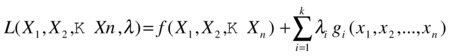
The extreme points are found by solving the system obtained by setting the components of the gradient vector of L to zero, that is, ∇ L(x1,x2,...,xn,λ) =(0,0,...,0). Which translates into:

By setting the partial derivatives to zero and solving the resulting system, we obtain the values of x1, x2,..., xn, λ1, λ2,...,λk corresponding to possible maxima and minima.
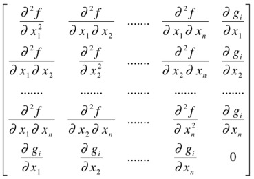
To determine the nature of the points (x1, x2,..., xn) found above, the following bordered Hessian matrix is used:
The nature of the extreme points can be determined by studying the set of bordered Hessian matrices:
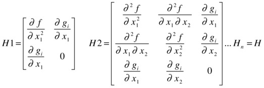
For a single restriction g1, if H1 < 0, H2 < 0, H3 < 0,..., H < 0, then the extreme point is a minimum.
For a single restriction g1, if H1 > 0, H2 < 0, H3 > 0, H4 < 0, H5 > 0, ... then the extreme point is a maximum.
For a collection of restrictions gi(x1,..., xn) (i = 1, 2,..., k) the lower right 0 will be a block of zeros and the conditions for a minimum will all have sign (-1)k, while the conditions for a maximum will have alternating signs with H1 having sign (-1)k+1. When considering several restrictions at the same time, it is easier to determine the nature of the extreme point by simple inspection.”
As an example we find and classify the extreme points of the function:
![]()
subject to the restriction:
![]()
First we find the Lagrangian L, which is a linear combination of the objective function and the constraints:
>> syms x y z L p
>> f = x + z

f =

x + z

>> g = x ^ 2 + y ^ 2 + z ^ 2-1

g =

x ^ 2 + y ^ 2 + z ^ 2 - 1

>> L = f + p * g

L =

x + z + p *(x^2 + y^2 + z^2-1)
Then, the possible extreme points are obtained by solving the system obtained by setting the components of the gradient vector of L equal to zero, that is, Ñ L(x1,x2,...,xn,λ) =(0,0,...,0). Which translates into:
>> [x, y, z, p] = solve (diff(L,x), diff(L,y), diff(L,z), diff(L,p), x, y, z, p)

x =

 -2^(1/2)/2
  2^(1/2)/2

y =

  2^(1/2)/2
 -2^(1/2)/2

z =

 0
 0

p =

  2^(1/2)/2
 -2^(1/2)/2
By matching all the partial derivatives to zero and solving the resulting system, we find the values of x1, x2,..., xn, λ1, λ2,...,λk corresponding to possible maxima and minima.
We already see that the possible extreme points are:
(-√2/2, √2/2, 0) and (√2/2, -√2/2, 0)
Now, let us determine the nature of these extreme points. To this end, we substitute them into the objective function.
>> clear all
>> syms x y z
>> f=x+z

f =

x + z

>> subs(f, {x,y,z},{-sqrt(2)/2,sqrt(2)/2,0})

ans =

   -0.7071

>> subs(f, {x,y,z},{sqrt(2)/2,-sqrt(2)/2,0})

ans =

    0.7071
Thus, at the point (-√2/2, √2/2, 0) the function has a maximum, and at the point (√2/2, -√2/2, 0) the function has a minimum.”
Here we shall introduce four classical theorems of differential calculus in several variables: the chain rule or composite function theorem, the implicit function theorem, the inverse function theorem and the change of variables theorem.
Consider a function ![]() : Rm→ Rn:
: Rm→ Rn:
(x1, x2,..., xm) → [F1(x1, x2,..., xm),...,Fn(x1, x2,..., xm)]
The vector function ![]() is said to be differentiable at the point a = (a1,...,am) if each of the component functions F1, F2,..., Fn is differentiable.
is said to be differentiable at the point a = (a1,...,am) if each of the component functions F1, F2,..., Fn is differentiable.
The Jacobian matrix of the above function is defined as:
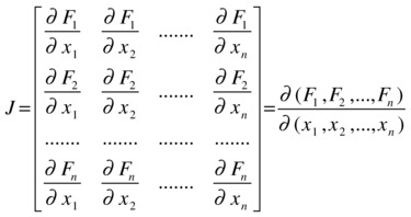
The Jacobian of a vector function is an extension of the concept of a partial derivative for a single-component function. MATLAB has the command jacobian which enables you to calculate the Jacobian matrix of a function.
As a first example, we calculate the Jacobian of the vector function mapping (x,y,z) to (x * y * z, y, x + z).
>> syms x y z
>> jacobian([x*y*z; y; x+z],[x y z])

ans =

[y * z, x * z, x * y]
[    0,     1,     0]
[    1,     0,     1]
As a second example, we calculate the Jacobian of the vector function ![]() at the point (0, -π / 2, 0).
at the point (0, -π / 2, 0).
>> syms x y z

>> J = jacobian ([exp(x), cos(y), sin(z)], [x, y, z])

J =

[exp(x), 0, 0]
[0,-sin(y), 0]
[0, 0, cos(z)]

>> subs(J,{x,y,z},{0,-pi/2,0})

ans =

    1 0 0
    0 1 0
    0 0 1
Thus the Jacobian turns out to be the identity matrix.
The Composite Function Theorem
The chain rule or composite function theorem allows you to differentiate compositions of vector functions. The chain rule is one of the most familiar rules of differential calculus. It is often first introduced in the case of single variable real functions, and is then generalized to vector functions. It says the following:
Suppose we have two vector functions
![]()
where U and V are open and consider the composite function ![]() .
.
If ![]() is differentiable at
is differentiable at ![]() and
and ![]() is differentiable at
is differentiable at ![]() , then
, then ![]() is differentiable at
is differentiable at ![]() and we have the following:
and we have the following:
![]()
MATLAB will directly apply the chain rule when instructed to differentiate composite functions.
Let us take for example ![]() and
and ![]() . If
. If ![]() we calculate the Jacobian of g at (0, 0) as follows.
we calculate the Jacobian of g at (0, 0) as follows.
>> syms x y u
>> f = x ^ 2 + y

f =

x ^ 2 + y

>> h = [sin(3*u), cos(8*u)]

h =

[sin(3*u), cos(8*u)]

>> g = compose (h, f)

g =

[sin(3*x^2 + 3*y), cos(8*x^2 + 8*y)]

>> J = jacobian(g,[x,y])

J =

[6 * x * cos(3*x^2 + 3*y), 3 * cos(3*x^2 + 3*y)]
[- 16 * x * sin(8*x^2 + 8*y), - 8 * sin(8*x^2 + 8*y)]

>> H = subs(J,{x,y},{0,0})

H =

0  3
0  0
Consider the vector function ![]() : A Ì Rn + m→ Rm where A is an open subset of Rn + m
: A Ì Rn + m→ Rm where A is an open subset of Rn + m
![]()
If Fi (i = 1, 2,..., m) are differentiable with continuous derivatives up to order r and the Jacobian matrix J = ∂ (F1,..., Fm) / ∂ (y1,..., ym) has non-zero determinant at a point ![]() such that
such that ![]() , then there is an open UÌRn containing
, then there is an open UÌRn containing ![]() and an open VÌ Rm containing
and an open VÌ Rm containing ![]() to and a single-valued function
to and a single-valued function ![]() : U→ V such that
: U→ V such that ![]() ∀ x ÎU and
∀ x ÎU and ![]() is differentiable of order r with continuous derivatives.
is differentiable of order r with continuous derivatives.
This theorem guarantees the existence of certain derivatives of implicit functions. MATLAB allows differentiation of implicit functions and offers the results in those cases where the hypotheses of the theorem are met.
As an example we will show that near the point (x, y, u, v) = (1,1,1,1) the following system has a unique solution:
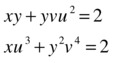
where u and v are functions of x and y (u = u(x, y), v = v(x, y)).
First, we check if the hypotheses of the implicit function theorem are met at the point (1,1,1,1).
The functions are differentiable and have continuous derivatives. We need to show that the corresponding Jacobian determinant is non-zero at the point (1,1,1,1).
>> clear all
>> syms x y u v
>> f = x * y + y * v * u ^ 2-2

f =

v * y * u ^ 2 + x * y - 2

>> g = x * u ^ 3 + y ^ 2 * v ^ 4-2

g =

x * u ^ 3 + v ^ 4 * y ^ 2 - 2

>> J = simplify (jacobian([f,g],[u,v]))

J =

[2 * u * v * y, u ^ 2 * y]
[3 * u ^ 2 * x, 4 * v ^ 3 * y ^ 2]

>> D = det (subs(J,{x,y,u,v},{1,1,1,1}))

D =

     5
Consider the vector function ![]() : U Ì Rn→ Rn where U is an open subset of Rn
: U Ì Rn→ Rn where U is an open subset of Rn
(x1, x2,..., xn) → [f1(x1, x2,..., xn),...,fn(x1, x2,..., xn)]
and assume it is differentiable with continuous derivative.
If there is an ![]() such that |J| = |∂(f1,...,fn) / ∂(x1,...,xn)| ≠ 0 at x0, then there is an open set A containing
such that |J| = |∂(f1,...,fn) / ∂(x1,...,xn)| ≠ 0 at x0, then there is an open set A containing ![]() and an open set B containing
and an open set B containing ![]() such that
such that ![]() and
and ![]() has an inverse function
has an inverse function ![]() that is differentiable with continuous derivative. In addition we have:
that is differentiable with continuous derivative. In addition we have:
![]() and if J = ∂ (f1,..., fn) / ∂ (x1,..., xn) then |J-1| = 1 / |J|.
and if J = ∂ (f1,..., fn) / ∂ (x1,..., xn) then |J-1| = 1 / |J|.
MATLAB automatically performs the calculations related to the inverse function theorem, provided that the assumptions are met.
As an example, we consider the vector function (u(x, y), v(x, y)), where:
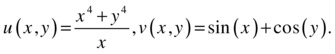
We will find the conditions under which the vector function (x(u,v), y(u,v)) is invertible, with x = x (u, v) and y = y(u,v), and find the derivative and the Jacobian of the inverse transformation. We will also find its value at the point (π/4,-π/4).
The conditions that must be met are those described in the hypotheses of the inverse function theorem. The functions are differentiable with continuous derivatives, except perhaps at x= 0. Now let us consider the Jacobian of the direct transformation ∂ (u(x, y), v(x,y)) /∂(x, y):
>> syms x y
>> J = simple ((jacobian ([(x^4+y^4)/x, sin(x) + cos(y)], [x, y])))

J =

[3 * x ^ 2-1/x ^ 2 * y ^ 4, 4 * y ^ 3/x]
[cos(x),-sin(y)]

>> pretty(det(J))

                               4          4     3
                     3 sin(y) x - sin(y) y + 4 y cos (x) x
                   - ---------------------------------------
                                        2
                                       x
Therefore, at those points where this expression is non-zero, we can solve for x and y in terms of u and v. In addition, it must be true that x π 0.
We calculate the derivative of the inverse function. Its value is the inverse of the initial Jacobian matrix and its determinant is the reciprocal of the determinant of the initial Jacobian matrix:
>> I=simple(inv(J));
>> pretty(simple(det(I)))

                                        2
                                       x
                   - ---------------------------------------
                               4          4     3
                     3 sin(y) x - sin(y) y + 4 y cos (x) x
Observe that the determinant of the Jacobian of the inverse vector function is indeed the reciprocal of the determinant of the Jacobian of the original function.
We now find the value of the inverse at the point (π/4,-π/4):
>> numeric(subs(subs(determ(I),pi/4,'x'),-pi/4,'y'))

ans =

   0.38210611216717

>> numeric(subs(subs(symdiv(1,determ(J)),pi/4,'x'),-pi/4,'y'))

ans =

   0.38210611216717
Again these results confirm that the determinant of the Jacobian of the inverse function is the reciprocal of the determinant of the Jacobian of the function.
The Change of Variables Theorem
The change of variable theorem is another key tool in multivariable differential analysis. Its applications extend to any problem in which it is necessary to transform variables.
Suppose we have a function f(x,y) that depends on the variables x and y, and that meets all the conditions of differentiation and continuity necessary for the inverse function theorem to hold. We introduce new variables u and v, relating to the above, regarding them as functions u = u(x,y) and v = v(x,y), so that u and v also fulfill the necessary conditions of differentiation and continuity (described by the inverse function theorem) to be able to express x and y as functions of u and v: x=x (u,v) and y=y(u,v).
Under the above conditions, it is possible to express the initial function f as a function of the new variables u and v using the expression:
f(u,v) = f (x(u,v), y(u,v))|J| where J is the Jacobian ∂ (x (u, v), y(u,v)) /∂(u, v).
The theorem generalizes to vector functions of n components.
As an example we consider the function ![]() and the transformation u = u(x,y) = x + y, v = v(x,y) = x to finally find f(u,v).
and the transformation u = u(x,y) = x + y, v = v(x,y) = x to finally find f(u,v).
We calculate the inverse transformation and its Jacobian to apply the change of variables theorem:
>> syms x y u v
>> [x, y] = solve('u=x+y,v=x','x','y')

x =

v

y =

u-v

>> jacobian([v,u-v],[u,v])

ans =

[0,   1]
[1, - 1]

>> f = exp(x-y);
>> pretty (simple (subs(f,{x,y},{v,u-v}) * abs (det (jacobian ()))
   ((([v, u-v], [u, v])))

                                 exp(2 v-u)
The requested function is f(u,v) = e2v-u.
Series Expansions in Several Variables
The familiar concept of a power series representation of a function of one variable can be generalized to several variables. Taylor’s theorem for several variables theorem reads as follows:
Let ![]() , (x1,...,xn) → f(x1,...,xn), be differentiable k times with continuous partial derivatives.
, (x1,...,xn) → f(x1,...,xn), be differentiable k times with continuous partial derivatives.
The Taylor series expansion of order k of ![]() at the point
at the point ![]() is as follows:
is as follows:
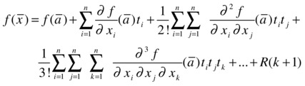
Here ![]()
R = remainder.
Normally, the series are given up to order 2.
As an example we find the Taylor series up to order 2 of the following function at the point (1,0):
![]()
>> pretty(simplify(subs(f,{x,y},{1,0})+subs(diff(f,x),{x,y},{1,0})*(x-1)
+subs(diff(f,y),{x,y},{1,0})*(y)+1/2*(subs(diff(f,x,2),{x,y},{1,0})* (x-1)^2+subs(diff(f,x,y),{x,y},{1,0})*(x-1)*(y)+ subs(diff(f,y,2),{x,y},{1,0})* (y)^2)))

              2
         2   y
  (x - 1)   --- + 1
             2
Curl, Divergence and the Laplacian
The most common concepts used in the study of vector fields are directly treatable by MATLAB and are summarized below.
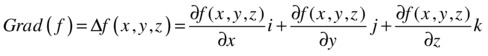
Definition of gradient: If h = f(x,y,z), then the gradient of f, which is denoted by D f(x, y, z), is the vector:
Definition of a scalar potential of a vector field: A vector field ![]() is called conservative if there is a differentiable function f such that
is called conservative if there is a differentiable function f such that ![]() . The function f is known as a scalar potential function for
. The function f is known as a scalar potential function for ![]() .
.
Definition of the curl of a vector field: The curl of a vector ![]() field is the following:
field is the following:
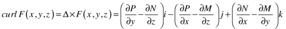
Definition of a vector potential of a vector field: A vector field F is a vector potential of another vector field G if F = curl (G).
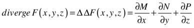
Definition of the divergence of a vector field: The divergence of the vector field ![]() is the following:
is the following:
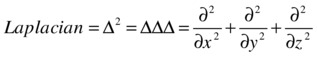
Definition of the Laplacian: The Laplacian is the differential operator defined by:
As a first example, we calculate gradient and Laplacian of the function:
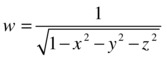
>> gradient=simplify([diff(f,x), diff(f,y), diff(f,z)])

gradient =

[x /(-x^2-y^2-z^2 + 1) ^(3/2), y /(-x^2-y^2-z^2 + 1) ^(3/2), z /(-x^2-y^2-z^2 + 1) ^(3/2)]

>> pretty (gradient)

  +-                                                                     -+
  |            x                      y                      z            |
  |  ---------------------, ---------------------, ---------------------  |
  |                      3                      3                      3  |
  |                      -                      -                      -  |
  |                      2                      2                      2  |
  |      2    2    2            2    2    2            2    2    2        |
  |  (- x  - y  - z  + 1)   (- x  - y  - z  + 1)   (- x  - y  - z  + 1)   |
  +-                                                                     -+

>> Laplacian = simplify ([diff(f,x,2) + diff(f,y,2) + diff(f,z,2)])

Laplacian =

3 /(-x^2-y^2-z^2 + 1) ^(5/2)

>> pretty (Laplacian)

            3
  ---------------------
                      5
                      -
                      2
      2    2    2
  (- x  - y  - z  + 1)
As a second example, we calculate the curl and the divergence of the vector field:
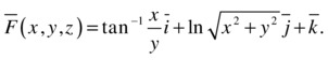
>> M = atan (x/y)

M =

atan (x/y)

>> N = log (sqrt(x^2+y^2))

N =

log ((x^2 + y^2) ^(1/2))

>> P = 1

P =
     1

>> Curl = simplify ([diff(P,y)-diff(N,z), diff(P,x)-diff(M,z), diff(N,x)-diff(M,y)])

Curl =

[0, 0, (2 * x) /(x^2 + y^2)]

>> pretty (Curl)

  +-               -+
  |          2 x    |
  |  0, 0, -------  |
  |         2   2   |
  |        x + y    |
  +-               -+

>> Divergence = simplify (diff(M,x) + diff(N,y) + diff(P,z))

Divergence =

(2 * y) /(x^2 + y^2)

>> pretty (divergence)

    2 y
  -------
   2   2
  x + y
Rectangular, Spherical and Cylindrical Coordinates
MATLAB allows you to easily convert cylindrical and spherical coordinates to rectangular, cylindrical to spherical coordinates, and their inverse transformations. As the cylindrical and spherical coordinates, we have the following:
In a cylindrical coordinate system, a point P in the space is represented by a triplet (r, θ, z), where:
- r is the distance from the origin (O) to the projection P' of P in the XY plane
- θ is the angle between the X axis and the segment OP'
- z is the distance PP'
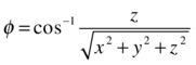
In a spherical coordinate system, a point P in the space is represented by a triplet (ρ, θ, φ), where:
- ρ is the distance from P to the origin
- θ is the same angle as the one used in cylindrical coordinates
- φ is the angle between the positive Z axis and the segment OP
The following conversion equations are easily found:
Cylindrical to rectangular:
![]()
![]()
![]()
Rectangular to cylindrical:
![]()

![]()
Spherical to rectangular:
![]()
![]()
![]()
Rectangular to spherical:
![]()

As a first example we express the surfaces with equations given by xz = 1 and x2 + y2 + z2 = 1 in spherical coordinates.
>> clear all
>> syms x y z r t a
>> f = x * z-1

f =

x * z - 1

>> equation = simplify (subs (f, {x, y, z}, {r * sin(a) * cos(t), r * sin(a) * sin(t), r * cos(a)}))

equation =

r ^ 2 * cos(a) * sin(a) * cos(t) - 1

>> pretty (equation)

   2
  r cos(a) sin(a) cos(t) - 1

g =

x ^ 2 + y ^ 2 + z ^ 2 - 1

>> equation1 = simplify (subs (g, {x, y, z}, {r * sin(a) * cos(t), r * sin(a) * sin(t), r * cos(a)}))

equation1 =

r ^ 2 - 1

>> pretty (equation1)

   2
  r -1
However, MATLAB provides commands that allow you to transform between different coordinate systems.
Below are the basic MATLAB commands which can be used for coordinate transformation.
|
[RHO, THETA, Z] = cart2ctl (X, Y, Z) [RHO, THETA] = cart2pol(X,Y) |
Transforms Cartesian coordinates to cylindrical coordinates Transforms Cartesian coordinates to polar coordinates |
|
[THETA, PHI, R] = cart2sph (X, Y, Z) |
Transforms Cartesian coordinates to spherical coordinates |
|
[X, Y, Z] = pol2cart (RHO, THETA, Z) [X, Y] = pol2cart (RHO, THETA) |
Transforms Cartesian coordinates to cylindrical coordinates Transforms polar coordinates to Cartesian coordinates |
|
[x, y, z] = sph2cart (THETA, PHI, R) |
Transforms spherical coordinates to Cartesian coordinates |
The following example transforms the point (π1, 2) in polar coordinates to Cartesian coordinates.
>> [X, Y, Z] = pol2cart(pi,1,2)

X =

    -1

Y =

  1. 2246e-016

Z =

     2
Next we transform the point (1,1,1) in Cartesian coordinates to spherical and cylindrical coordinates.
>> [X, Y, Z] = cart2sph(1,1,1)

X =

    0.7854

Y =

    0.6155

Z =

    1.7321

>> [X, Y, Z] = cart2pol(1,1,1)

X =

    0.7854

Y =

    1,4142

Z =

     1
The following example transforms the point (2,π/4) in polar coordinates into Cartesian coordinates.
>> [X, Y] = pol2cart(2,pi/4)

X =

   -0.3268

Y =

    0.7142
EXERCISE 7-1
Study the differentiability of the function:
 if
if ![]() and
and ![]() if
if ![]() .
.
We begin by studying the continuity of the function at the point x = 0.
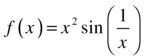
>> syms x
>> f = x ^ 2 * sin(1/x)
f =
x ^ 2 * sin(1/x)
>> limit(f,x,0, 'right')
ans =
0
>> limit(f,x,0, 'left')
ans =
0
>>
>> limit(f,x,0)
ans =
0
We see that the function is continuous at x = 0 because the limit of the function as x tends to zero coincides with the value of the function at zero. It may therefore be differentiable at zero.
We now determine whether the function is differentiable at the point x = 0:
>> syms h, limit((h^2*sin(1/h) - 0)/h,h,0)
ans =
0
Thus, we see that:
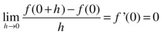
which indicates that the function f is differentiable at the point x = 0.
Let us now see what happens at a non-zero point x = a:
>> pretty(simple(limit((subs(f,{x},{a+h})-subs(f,{x},{a}))/h,h,a)))
/ 1 / 1
4-sin | --- | -a sin| -- |
2 a / a /
Thus, we conclude that:
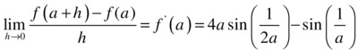
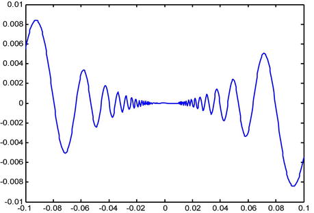
Thus, we have already found the value of the derivative at any non-zero point x = a. We represent the function in the figure below.
>> fplot ('x ^ 2 * sin (x)', [-1/10,1/10])
EXERCISE 7-2
Calculate the derivative with respect to x of the following functions:
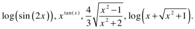
>> pretty(simple(diff('log(sin(2*x))','x')))
2 cot(2 x)
>> pretty(simple(diff('x^tanx','x')))
tanx
x tanx
------------
x
>> pretty(simple(diff('(4/3)*sqrt((x^2-1)/(x^2+2))','x')))
x
4 -----------------------
2 1/2 2 3/2
(x - 1) (x + 2)
>> pretty(simple(diff('log(x+(x^2+1)^(1/2))','x')))
1
------------
2 1/2
(x + 1)
EXERCISE 7-3
Calculate the nth derivative of the following functions:
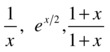
>> f='1/x';
>> [diff(f),diff(f,2),diff(f,3),diff(f,4),diff(f,5)]
ans =
-1/x ^ 2 2/x ^ 3 -6/x ^ 4 24/x ^ 5 -120/x ^ 6
We begin to see the pattern emerging, so the nth derivative is given by

>> f='exp(x/2)';
>> [diff(f),diff(f,2),diff(f,3),diff(f,4),diff(f,5)]
ans =
1/2*exp(1/2*x) 1/4*exp(1/2*x) 1/8*exp(1/2*x) 1/16*exp(1/2*x 1/32*exp(1/2*x)
Thus the nth derivative is ![]() .
.
>> f='(1+x)/(1-x)';
>> [simple(diff(f)),simple(diff(f,2)),simple(diff(f,3)),simple(diff(f,4))]
ans =
2 /(-1+x) ^ 2-4 /(-1+x) ^ 3 12 /(-1+x) ^ 4-48 /(-1+x) ^ 5
Thus, the nth derivative is equal to  .
.
EXERCISE 7-4
Find the equation of the tangent to the curve ![]() at x = -1.
at x = -1.
Also find the x for which the tangents to the curve are 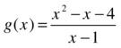 horizontal and vertical. Find the asymptotes.
>> f ='2 * x ^ 3 + 3 * x ^ 2-12 * x + 7';
>> g = diff (f)
g =
6*x^2+6*x-12
>> subs(g,-1)
ans =
-12
>> subs(f,-1)
ans =
20
We see that the slope of the tangent line at the point x = -1 is -12, and the function has value 20 at x = -1. Therefore the equation of the tangent to the curve at the point (-1,20) will be:
y - 20 = -12 (x - (-1))
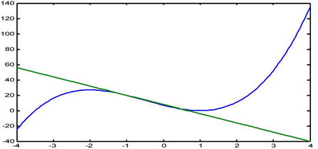
We graphically represent the curve and its tangent on the same axes.
>> fplot('[2*x^3+3*x^2-12*x+7, 20-12*(x - (-1))]',[-4,4])
To calculate the horizontal tangent to the curve y = f(x) at x= x0, we find the values x0 for which the slope of the tangent is zero (f'(x0) = 0). The equation of this tangent will therefore be y = f(x0).
To calculate the vertical tangents to the curve y = f (x) at x = x0, we find the values x0 which make the slope of the tangent infinite (f'(x0) = ∞). The equation of this tangent will then be = x0:
>> g ='(x^2-x+4) /(x-1)'
>> solve(diff(g))
ans =
[ 3]
[-1]
>> subs(g,3)
ans =
5
>> subs(g,-1)
ans =
-3
The two horizontal tangents have equations:
y = g’ [-1](x + 1) - 3, that is, y = -3.
y = g’[3](x - 3) +5, that is, y = 5.
The horizontal tangents are not asymptotes because the corresponding values of x0 are finite (-1 and 3).
We now consider the vertical tangents. To do this, we calculate the values of x that make g ' (x) infinite (i.e. values for which the denominator of g ' is zero, but do not cancel with the numerator):
>> solve('x-1')
ans =
1
Therefore, the vertical tangent has equation x = 1.
For x = 1, the value of g (x) is infinite, so the vertical tangent is a vertical asymptote.
subs(g,1)
Error, division by zero
Indeed, the line x = 1 is a vertical asymptote.
As ![]() , there are no horizontal asymptotes.
, there are no horizontal asymptotes.
Now let’s see if there are any oblique asymptotes:
>> syms x,limit(((x^2-x+4)/(x-1))/x,x,inf)
ans =
1
>> syms x,limit(((x^2-x+4)/(x-1) - x)/x,x,inf)
ans =
0
Thus, there is an oblique asymptote y = x.
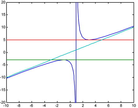
We now graph the curve with its asymptotes and tangents:
On the same axes (see the figure below) we graph the curve whose equation is g(x) = (x2-x + 4)/(x-1), the horizontal tangents with equations a(x) = -3 and b(x) = 5, the oblique asymptote with equation c(x) = x and the horizontal and vertical asymptotes (using the default command fplot ):
>> fplot('[(x^2-x+4)/(x-1),-3,5,x]',[-10,10,-20,20])
EXERCISE 7-5
Decompose a positive number a as a sum of two summands so that the sum of their cubes is minimal.
Let x be one of the summands. The other will be a-x. We need to minimize the sum x3+ (a-x)3.
>> syms x a;
>> f='x^3+(a-x)^3'
f =
x^3+(a-x)^3
>> solve(diff(f,'x'))
ans =
1/2 * a
The possible maximum or minimum is at x = a/2. We use the second derivative to see that it is indeed a minimum:
>> subs(diff(f,'x',2),'a/2')
ans =
3 * a
As a > 0 (by hypothesis), 4a > 0, which ensures the existence of a minimum at x = a/2.
Therefore x = a/2 and a-x = a-a/2= a/2. That is, we obtain a minimum when the two summands are equal.
EXERCISE 7-6
Suppose you want to purchase a rectangular plot of 1600 square meters and then fence it. Knowing that the fence costs 200 cents per meter, what dimensions must the plot of land have to ensure that the fencing is most economical?
If the surface area is 1600 square feet and one of its dimensions, unknown, is x, the other will be 1600/x.
The perimeter of the rectangle is ![]() , and the cost is given by
, and the cost is given by ![]() :
:
>> f ='200 * (2 * x + 2 *(1600/x))'
f =
200 * (2 * x + 2 *(1600/x))
This is the function to minimize:
>> solve(diff(f))
ans =
[ 40]
[-40]
The possible maximum and minimum are presented for x = 40 and x = -40. We use the second derivative to determine their nature:
>> [subs(diff(f,2), 40), subs(diff(f,2), -40)]
ans =
20 - 20
x = 40 is a minimum, and x =-40 is a maximum. Thus, one of the sides of the rectangular field is 40 meters, and the other will measure 1,600/40 = 40 meters. Therefore the optimal rectangle is a square with sides of 40 meters.
EXERCISE 7-7
Given the function of two real variables defined by:
 if
if ![]() and
and ![]() if
if ![]()
calculate the partial derivatives of f at the origin. Study the differentiability of the function.
To find ∂f/∂x and ∂f/∂y at the point (0,0), we directly apply the definition of the partial derivative at a point:
>> syms x y h k
>> limit((subs(f,{x,y},{h,0})-0)/h,h,0)
ans =
0
>> limit((subs(f,{x,y},{0,k})-0)/k,k,0)
ans =
0
We see that the limits of the two previous expressions when ![]() and
and ![]() , respectively, are both zero. That is to say:
, respectively, are both zero. That is to say:
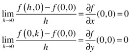
Thus the two partial derivatives have the same value, namely zero, at the origin.
But the function is not differentiable at the origin, because it is not continuous at (0,0), since it has no limit as ![]() :
:
>> syms m
>> limit((m*x)^2/(x^2+(m*x)^2),x,0)
ans =
m^2 /(m^2 + 1)
The limit does not exist at (0,0), because if we consider the directional limits with respect to the family of straight lines y = mx, the result depends on the parameter m.
EXERCISE 7-8
Find and classify the extreme points of the function
![]()
We begin by finding the possible extreme points. To do so, we equate each of the partial derivatives of the function with respect to each of its variables to zero (i.e. the components of the gradient vector of f) and solve the resulting system in three variables:
>> syms x y
>> f = -120 * x ^ 3-30 * x ^ 4 + 18 * x ^ 5 + 5 * x ^ 6 + 30 * x * y ^ 2
f =
5 * x ^ 6 + 18 * x ^ 5-30 * x ^ 4-120 * x ^ 3 + 30 * x * y ^ 2
>> [x y] = solve (diff(f,x), diff(f,y), x, y)
x =
0
2
-2
-3
y =
0
0
0
0
So the possible extreme points are: (- 2,0), (2,0), (0,0) and (-3,0).
We will analyze what kind of extreme points these are. To do this, we calculate the Hessian matrix and express it as a function of x and y.
>> clear all
>> syms x y
>> f=-120*x^3-30*x^4+18*x^5+5*x^6+30*x*y^2
f =
5*x^6 + 18*x^5 - 30*x^4 - 120*x^3 + 30*x*y^2
>> H=simplify([diff(f,x,2),diff(diff(f,x),y);diff(diff(f,y),x),diff(f,y,2)])
H =
[- 30 * x *(-5*x^3-12*x^2 + 12*x + 24), 60 * y]
[ 60*y, 60*x]
Now we calculate the value of the determinant of the Hessian matrix at the possible extreme points.
>> det(subs(H,{x,y},{0,0}))
ans =
0
The origin turns out to be a degenerate point, as the determinant of the Hessian matrix is zero at (0,0).
We will now look at the point (- 2,0).
>> det(subs(H,{x,y},{-2,0}))
ans =
57600
>> eig(subs(H,{x,y},{-2,0}))
ans =
-480
-120
The Hessian matrix at the point (-2,0) has non-zero determinant, and is also negative definite, because all its eigenvalues are negative. Therefore, the point (-2,0) is a maximum of the function.
We will now analyze the point (2,0).
>> det(subs(H,{x,y},{2,0}))
ans =
288000
>> eig(subs(H,{x,y},{2,0}))
ans =
120
2400
The Hessian matrix at the point (2,0) has non-zero determinant, and is furthermore positive definite, because all its eigenvalues are positive. Therefore, the point (2,0) is a minimum of the function.
We will now analyze the point (-3,0).
>> det(subs(H,{x,y},{-3,0}))
ans =
-243000
>> eig(subs(H,{x,y},{-3,0}))
ans =
-180
1350
The Hessian matrix at the point (-3,0) has non-zero determinant, and, in addition, is neither positive definite nor negative, because it has both positive and negative eigenvalues. Therefore, the point (-3,0) is a saddle point of the function.
EXERCISE 7-9
Find and classify the extreme points of the function:
![]()
subject to the restrictions: x2 +y2 = 16 and x + y + z = 10.
We first find the Lagrangian L, which is a linear combination of the objective function and the constraints:
>> clear all
>> syms x y z L p q
>> f =(x^2+y^2) ^(1/2)-z
f =
(x ^ 2 + y ^ 2) ^ (1/2) - z
>> g1 = x ^ 2 + y ^ 2 - 16, g2 = x + y + z - 10
G1 =
x ^ 2 + y ^ 2 - 16
G2 =
x + y + z - 10
>> L = f + p * g1 + q * g2
L =
(x ^ 2 + y ^ 2) ^ (1/2) - z + q *(x + y + z - 10) + p *(x^2 + y^2 - 16)
Then, the possible extreme points are found by solving the system obtained by setting the components of the gradient vector of L to zero, that is, ∇L(x1,x2,...,xn,λ) =(0,0,...,0). Which translates into:
>> [x, y z, p, q] = solve (diff(L,x), diff(L,y), diff(L,z), diff(L,p), diff(L,q), x, y z, p, q)
x =
-2 ^(1/2)/8 - 1/8
y =
1
z =
2 * 2 ^(1/2)
p =
2 * 2 ^(1/2)
q =
10 - 4 * 2 ^(1/2)
Matching all the partial derivatives to zero and solving the resulting system, we find the values of x1, x2,..., xn, λ1, λ2,...,λk corresponding to possible maxima and minima.
We already have one possible extreme point:
(-(1+√2)/8, 1, 2√2)
We need to determine what kind of extreme point this is. To this end, we substitute it into the objective function.
>> syms x y z
>> vpa (subs (f, {x, y, z}, {-2 ^(1/2)/8-1/8,1,2*2^(1/2)}))
ans =
-1.78388455796197398228741803905
Thus, at the point (-(1+√2)/8, 1/2√2), the function has a maximum.
EXERCISE 7-10
Given the function ![]() and the transformation u = u(x,y) = 2 x + y, v = v(x,y) = x – y, find f(u,v).
and the transformation u = u(x,y) = 2 x + y, v = v(x,y) = x – y, find f(u,v).
We calculate the inverse transformation and its Jacobian in order to apply the change of variables theorem:
>> [x, y] = solve('u=2*x+y,v=x-y','x','y')
x =
u + v/3
y =
u - (2 * v) / 3
>> jacobian([u/3 + v/3,u/3-(2*v)/3], [u, v])
ans =
[1/3, 1/3]
[1/3, 2/3]
>> f = 10 ^(x-y);
>> pretty (simple (subs(f,{x,y},{u/3 + v/3,u/3-(2*v)/3}) *))
abs (det (jacobian([u/3 + v/3,u/3-(2*v)/3], [u, v])))
v
10
---
3
Thus the requested function is f(u,v) = 10v/3.
EXERCISE 7-11
Find the Taylor series at the origin, up to order 2, of the function:
![]()
>> f = exp(x+y^2)
f =
>> pretty (simplify (subs(f,{x,y},{0,0}) + subs (diff(f,x), {x, y}, {0,0}) * (x) + subs (diff(f,y), {x, y}, {0,0}) * (y) + 1/2 * (subs (diff(f,x,2), {x, y}, {0,0}) * (x) ^ 2 + subs (diff(f,x,y), {x, y}, {0,0}) * (x) * (y) + subs (diff(f,y,2), {x, y}, {0,0}) * (y) ^ 2)))
2
x 2
-- + x + y + 1
2
EXERCISE 7-12
Express, in Cartesian coordinates, the surface which is given in cylindrical coordinates by z = r2 (1 + sin(t)).
>> syms x y z r t a
>> f = r ^ 2 * (1 + sin(t))
f =
r ^ 2 * (sin(t) + 1)
>> Cartesian = simplify(subs(f, {r, t}, {sqrt(x^2+y^2), bind(y/x)}))
Cartesian =
(x ^ 2 + y ^ 2) * (y / (x *(y^2/x^2 + 1) ^(1/2)) + 1)
>> pretty (Cartesian)
2 2 / y
(x + y ) | --------------- + 1 |
| / 2 1/2 |
| | y | |
| x | -- + 1 | |
| | 2 | |
x / /
EXERCISE 7-13
Find the unit tangent, the unit normal, and the unit binormal vectors of the twisted cubic: x = t, y = t2, z = t3.
We begin by restricting the variable t to the real field:
>> x = sym('x','real);
We define the symbolic vector V as follows:
>> syms t, V = [t,t^2,t^3]
V =
[t, t ^ 2, t ^ 3]
The tangent vector is calculated by:
>> tang = diff(V)
tang =
[1, 2 *, 3 * t ^ 2]
The unit tangent vector will be:
>> ut = simple (tang/sqrt(dot(tang,tang)))
tu =
[1/(1+4*t^2+9*t^4)^(1/2),2*t/(1+4*t^2+9*t^4)^(1/2),3*t^2/(1+4*t^2+9*t^4)^(1/2)]
To find the unit normal vector we calculate ((v'∧v'') ∧v')/(|v'∧v''| |v'|):
>> v1 = cross(diff(V),diff(V,2)) ;
>> nu = simple(cross(v1,tang)/(sqrt(dot(v1,v1))*sqrt(dot(tang,tang))))
nu =
[ (-2*t-9*t^3)/(9*t^4+9*t^2+1)^(1/2)/(1+4*t^2+9*t^4)^(1/2),
(1-9*t^4)/(9*t^4+9*t^2+1)^(1/2)/(1+4*t^2+9*t^4)^(1/2), (6*t^3+3*t)/(9*t^4+9*t^2+1)^(1/2)/(1+4*t^2+9*t^4)^(1/2)]
The unit binormal vector is the vector product of the tangent vector and the unit normal vector.
>> bu = simple(cross(tu,nu))
bu =
[3*t^2/(9*t^4+9*t^2+1)^(1/2),-3*t/(9*t^4+9*t^2+1)^(1/2),1/(9*t^4+9*t^2+1)^(1/2)]
The unit binormal vector can also be calculated via (v'∧v ") / |v'∧v" | as follows:
>> bu = simple(v1/sqrt(dot(v1,v1)))
bu =
[3*t^2/(9*t^4+9*t^2+1)^(1/2),-3*t/(9*t^4+9*t^2+1)^(1/2),1/(9*t^4+9*t^2+1)^(1/2)]
We have calculated the Frenet frame for a twisted cubic.