![]()
Differential Equations
First Order Differential Equations
Although it implements only a relatively small number of commands related to this topic, MATLAB’s treatment of differential equations is nevertheless very efficient. We shall see how we can use these commands to solve each type of differential equation algebraically. Numerical methods for the approximate solution of equations and systems of equations are also implemented.
The basic command used to solve differential equations is dsolve. This command finds symbolic solutions of ordinary differential equations and systems of ordinary differential equations. The equations are specified by symbolic expressions where the letter D is used to denote differentiation, or D2, D3, etc., to denote differentiation of order 2,3,..., etc. The letter preceded by D (or D2, etc.) is the dependent variable (which is usually y), and any letter that is not preceded by D (or D2, etc.) is a candidate for the independent variable. If the independent variable is not specified, it is taken to be x by default. If x is specified as the dependent variable, then the independent variable is t. That is, x is the independent variable by default, unless it is declared as the dependent variable, in which case the independent variable is understood to be t.
You can specify initial conditions using additional equations, which take the form y(a) = b or Dy(a) = b,..., etc. If the initial conditions are not specified, the solutions of the differential equations will contain constants of integration, C1, C2,..., etc. The most important MATLAB commands that solve differential equations are the following:
- dsolve(‘equation’, ‘v’): This solves the given differential equation, where v is the independent variable (if ‘v’ is not specified, the independent variable is x by default). This returns only explicit solutions.
- dsolve(‘equation’, ‘initial_condition’,..., ‘v’): This solves the given differential equation subject to the specified initial condition.
- dsolve(‘equation’, ‘cond1’, ‘cond2’,..., ‘condn’, ‘v’): This solves the given differential equation subject to the specified initial conditions.
- dsolve(‘equation’, ‘cond1, cond2,..., condn’, ‘v’): This solves the given differential equation subject to the specified initial conditions.
- dsolve(‘eq1’, ‘eq2’,..., ‘eqn’, ‘cond1’, ‘cond2’,..., ‘condn’ , ‘v’): This solves the given system of differential equations subject to the specified initial conditions.
- dsolve(‘eq1, eq2,..., eqn’, ‘cond1, cond2,..., condn’ , ‘v’): This solves the given system of differential equations subject to the specified initial conditions.
- maple(‘dsolve(equation, func(var))’): This solves the given differential equation, where var is the independent variable and func is the dependent variable (returns implicit solutions).
- maple(‘dsolve({equation, cond1, cond2,... condn}, func(var))’): This solves the given differential equation subject to the specified initial conditions.
- maple(‘dsolve({eq1, eq2,..., eqn}, {func1(var), func2(var),... funcn(var)})’): This solves the given system of differential equations (returns implicit solutions).
- maple(‘dsolve(equation, func(var), ‘explicit’)’): This solves the given differential equation, offering the solution in explicit form, if possible.
Examples are given below.
First, we solve differential equations of first order and first degree, both with and without initial values.
>> pretty(dsolve('Dy = a*y'))

  C2 exp(a t)

>> pretty(dsolve('Df = f + sin(t)'))

              sin(t)   cos(t)
  C6 exp(t) - ------ - ------
                2        2
The previous two equations can also be solved in the following way:
>> pretty(sym(maple('dsolve(diff(y(x), x) = a * y, y(x))')))

y(x) = exp(a x) _C1

>> pretty(maple('dsolve(diff(f(t),t)=f+sin(t),f(t))'))

f(t) = - 1/2 cos(t) - 1/2 sin(t) + exp(t) _C1

>> pretty(dsolve('Dy = a*y', 'y(0) = b'))

exp(a x) b

>> pretty(dsolve('Df = f + sin(t)', 'f(pi/2) = 0'))

     /   pi
  exp| - -- | exp(t)
        2  /          sin(t)   cos(t)
  ------------------ - ------ - ------
          2              2        2
Now we solve an equation of second degree and first order.
>> y = dsolve('(Dy) ^ 2 + y ^ 2 = 1', ' y(0) = 0', 's')

y =

 cosh((pi*i)/2 + s*i)
 cosh((pi*i)/2 - s*i)
We can also solve this in the following way:
>> pretty(maple('dsolve({diff(y(s),s)^2 + y(s)^2 = 1, y(0) = 0}, y(s))'))

y(s) = sin(s), y(s) = - sin(s)
Now we solve an equation of second order and first degree.
>> pretty(dsolve('D2y = - a ^ 2 * y ', 'y(0) = 1, Dy(pi/a) = 0'))

   exp(-a t i)   exp(a t i)
  ----------- + ----------
       2            2
Next we solve a couple of systems, both with and without initial values.
>> dsolve('Dx = y', 'Dy = -x')

ans =

     y: [1x1 sym]
     x: [1x1 sym]

>> y

y =

     cosh((pi*i)/2 + s*i)
     cosh((pi*i)/2 - s*i)

>> x

x =

x

>> y=dsolve('Df = 3*f+4*g', 'Dg = -4*f+3*g')

y =

     g: [1x1 sym]
     f: [1x1 sym]

>> y.g

ans =

     C27*cos(4*t)*exp(3*t) - C28*sin(4*t)*exp(3*t)

>> y.f

ans =

     C28*cos(4*t)*exp(3*t) + C27*sin(4*t)*exp(3*t)

>> y=dsolve('Df = 3*f+4*g, Dg = -4*f+3*g', 'f(0)=0, g(0)=1')

y =

     g: [1x1 sym]
     f: [1x1 sym]

>> y.g

ans =
     cos(4*t)*exp(3*t)

>> y.f

ans =
sin(4*t)*exp(3*t)
Numerical Solutions of Differential Equations
MATLAB provides commands in its Basic module allowing for the numerical solution of ordinary differential equations (ODEs), differential algebraic equations (DAEs) and boundary value problems. It is also possible to solve systems of differential equations with boundary values and parabolic and elliptic partial differential equations.
Ordinary Differential Equations with Initial Values
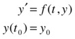
An ordinary differential equation contains one or more derivatives of the dependent variable y with respect to the independent variable t. A first order ordinary differential equation with an initial value for the independent variable can be represented as:
The previous problem can be generalized to the case where y is a vector, y = (y1, y2,..., yn).
MATLAB’s Basic module commands relating to ordinary differential equations and differential algebraic equations with initial values are presented in the following table:
|
Command |
Class of problem solving, numerical method and syntax |
|---|---|
|
ode45 |
Ordinary differential equations by the Runge–Kutta method |
|
ode23 |
Ordinary differential equations by the Runge–Kutta method |
|
ode113 |
Ordinary differential equations by Adams’ method |
|
ode15s |
Differential algebraic equations and ordinary differential equations using NDFs (BDFs) |
|
ode23s |
Ordinary differential equations by the Rosenbrock method |
|
ode23t |
Ordinary differential and differential algebraic equations by the trapezoidal rule |
|
ode23tb |
Ordinary differential equations using TR-BDF2 |
The common syntax for the previous seven commands is the following:
[T, y] = solver(odefun,tspan,y0)
[T, y] = solver(odefun,tspan,y0,options)
[T, y] = solver(odefun,tspan,y0,options,p1,p2...)
[T, y, TE, YE, IE] = solver(odefun,tspan,y0,options)
In the above, solver can be any of the commands ode45, ode23, ode113, ode15s, ode23s, ode23t, or ode23tb.
The argument odefun evaluates the right-hand side of the differential equation or system written in the form y' = f (t, y) or M(t, y)y '=f(t, y), where M(t, y) is called a mass matrix. The command ode23s can only solve equations with constant mass matrix. The commands ode15s and ode23t can solve algebraic differential equations and systems of ordinary differential equations with a singular mass matrix. The argument tspan is a vector that specifies the range of integration [t0, tf] (tspan= [t0, t1,...,tf], which must be either an increasing or decreasing list, is used to obtain solutions for specific values of t).The argument y0 specifies a vector of initial conditions. The arguments p1, p2,... are optional parameters that are passed to odefun. The argument options specifies additional integration options using the command options odeset which can be found in the program manual. The vectors T and y present the numerical values of the independent and dependent variables for the solutions found.
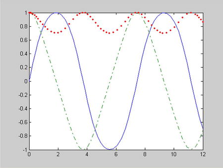
As a first example we find solutions in the interval [0,12] of the following system of ordinary differential equations:
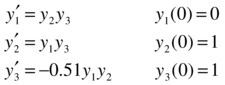
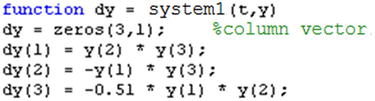
For this, we define a function named system1 in an M-file, which will store the equations of the system. The function begins by defining a column vector with three rows which are subsequently assigned components that make up the syntax of the three equations (Figure 9-1).
We then solve the system by typing the following in the Command Window:
>> [T, Y] = ode45(@system1,[0 12],[0 1 1])

T =

      0
   0.0001
   0.0001
   0.0002
   0.0002
   0.0005
   .
   .
   11.6136
   11.7424
   11.8712
   12.0000

Y =
   0 1.0000 1.0000
   0.0001 1.0000 1.0000
   0.0001 1.0000 1.0000
   0.0002 1.0000 1.0000
   0.0002 1.0000 1.0000
   0.0005 1.0000 1.0000
   0.0007 1.0000 1.0000
   0.0010 1.0000 1.0000
   0.0012 1.0000 1.0000
   0.0025 1.0000 1.0000
   0.0037 1.0000 1.0000
   0.0050 1.0000 1.0000
   0.0062 1.0000 1.0000
   0.0125 0.9999 1.0000
   0.0188 0.9998 0.9999
   0.0251 0.9997 0.9998
   0.0313 0.9995 0.9997
   0.0627 0.9980 0.9990
   .
   .
   0.8594-0.5105 0.7894
   0.7257-0.6876 0.8552
   0.5228-0.8524 0.9281
   0.2695-0.9631 0.9815
   -0.0118-0.9990 0.9992
   -0.2936-0.9540 0.9763
   -0.4098-0.9102 0.9548
   -0.5169-0.8539 0.9279
   -0.6135-0.7874 0.8974
   -0.6987-0.7128 0.8650
To better interpret the results, the above numerical solution can be graphed (Figure 9-2) by using the following syntax:
>> plot(T, Y(:,1), '-', T, Y(:,2),'-', T, Y(:,3),'. ')
Ordinary Differential Equations with Boundary Values
MATLAB also allows you to solve ordinary differential equations with boundary conditions. The boundary conditions specify a relationship that must hold between the values of the solution function at the end points of the interval on which it is defined. The simplest problem of this type is the system of equations
![]()
where x is the independent variable, y is the dependent variable and y' is the derivative with respect to x (i.e., y'= dy/dx). In addition, the solution on the interval [a, b] has to meet the following boundary condition:
![]()
More generally this type of differential equations can be expressed as follows:
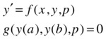
where the vector p consists of parameters which have to be determined simultaneously with the solution via the boundary conditions.
The command that solves these problems is bvp4c, whose syntax is as follows:
Sol = bvp4c(odefun, bcfun, solinit)
Sol = bvp4c(odefun, bcfun, solinit, options)
Sol = bvp4c(odefun, bcfun, solinit, options, p1,p2...)
In the syntax above odefun is a function that evaluates f (x, y). It may take one of the following forms:
dydx = odefun(x,y)
dydx = odefun(x,y,p1,p2,...)
dydx = odefun(x,y,parameters)
dydx = odefun(x,y,parameters,p1,p2,...)
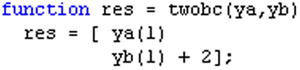
The argument bcfun in bvp4c is a function that computes the residual in the boundary conditions. Its form is as follows:
Res = bcfun(ya, yb)
Res = bcfun(ya,yb,p1,p2,...)
Res = bcfun(ya, yb,parameters)
Res = bcfun(ya,yb,parameters,p1,p2,...)
The argument solinit is a structure containing an initial guess of the solution. It has the following fields: x (which gives the ordered nodes of the initial mesh so that the boundary conditions are imposed at a = solinit.x(1) and b = solinit.x(end)); and y (the initial guess for the solution, given as a vector, so that the i-th entry is a constant guess for the i-th component of the solution at all the mesh points given by x). The structure solinit is created using the command bvpinit. The syntax is solinit = bvpinit(x,y).
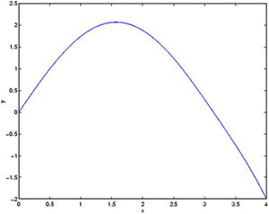
As an example we solve the second order differential equation:
![]()
whose solutions must satisfy the boundary conditions:

The previous problem is equivalent to the following:

We consider a mesh of five equally spaced points in the interval [0,4] and our initial guess for the solution is y1 = 1 and y2 = 0. These assumptions are included in the following syntax:
>> solinit = bvpinit (linspace (0,4,5), [1 0]);
The M-files depicted in Figures 9-3 and 9-4 show how to enter the equation and its boundary conditions.
The following syntax is used to find the solution of the equation:
>> Sun = bvp4c(@twoode, @twobc, solinit);
The solution can be graphed (Figure 9-5) using the command bvpval as follows:
>> y = bvpval(Sun, linspace(0.4));
>> plot(x, y(1,:));
Partial Differential Equations
MATLAB’s Basic module has features that enable you to solve partial differential equations and systems of partial differential equations with initial boundary conditions. The basic function used to calculate the solutions is pdepe, and the basic function used to evaluate these solutions is pdeval.
The syntax of the function pdepe is as follows:
Sol = pdepe(m, pdefun, icfun, bcfun, xmesh, tspan)
Sol = pdepe(m, pdefun, icfun, bcfun, xmesh, tspan, options)
Sun = pdepe(m,pdefun,icfun,bcfun,xmesh,tspan,options,p1,p2...)
The parameter m takes the value 0, 1 or 2 according to the nature of the symmetry of the problem (block, cylindrical or spherical, respectively). The argument pdefun defines the components of the differential equation, icfun defines the initial conditions, bcfun defines the boundary conditions, xmesh and tspan are vectors [x0, x1,...,xn] and [t0, t1,...,tf] that specify the points at which a numerical solution is requested (n, f≥ 3), options specifies some calculation options of the underlying solver (RelTol, AbsTol,NormControl, InitialStep and MaxStep to specify relative tolerance, absolute tolerance, norm tolerance, initial step and max step, respectively) and p1, p2,... are parameters to pass to the functions pdefun, icfun and bcfun.
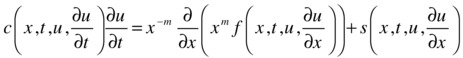
pdepe solves partial differential equations of the form:
where a≤ x≤ b and t0≤ t £ tf. Moreover, for t = t0 and for all x the solution components meet the initial conditions:
![]()
and for all t and each x = a or x = b, the solution components satisfy the boundary conditions of the form:
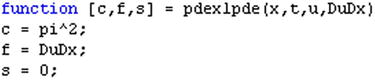
In addition, we have that a = xmesh (1), b = xmesh (end), tspan (1) = t0 and tspan (end) = tf. Moreover pdefun finds the terms c, f and s of the partial differential equation, so that:
- [f, s] = pdefun(x, t, u, dudx)
Similarly icfun evaluates the initial conditions
- u = icfun(x)
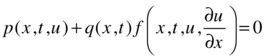
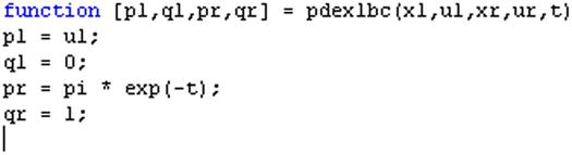
Finally, bcfun evaluates the terms p and q of the boundary conditions:
- [pl, ql, pr, qr] = bcfun(xl, ul, xr, ur, t)
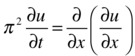
As a first example, we solve the following partial differential equation (xÎ[0,1] and t≥ 0):
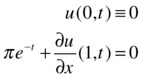
satisfying the initial condition:
![]()
and the boundary conditions:
We begin by defining functions in M-files as shown in Figures 9-6 to 9-8.
![]()
Figure 9-7.
Once the support functions have been defined, we define the function that solves the equation (see the M-file in Figure 9-9).
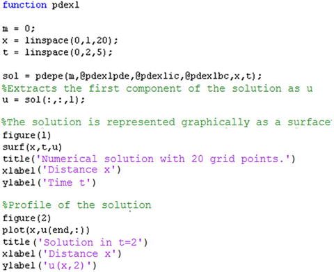
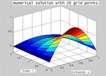
To view the solution (Figures 9-10 and 9-11), we enter the following into the MATLAB Command Window:
>> pdex1
As a second example, we solve the following system of partial differential equations (xÎ[0,1] and t³ 0):
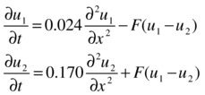
![]()
satisfying the initial conditions:

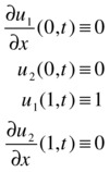
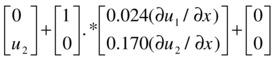
and the boundary conditions:
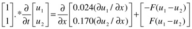
To conveniently use the function pdepe, the system can be written as:
The left boundary condition can be written as:
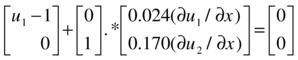
and the right boundary condition can be written as:
We start by defining the functions in M-files as shown in Figures 9-12 to 9-14.
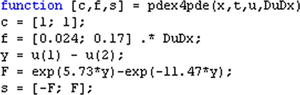
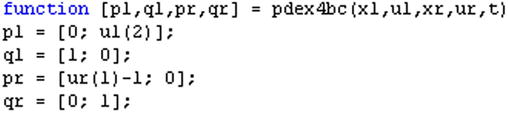
Figure 9-13.
Once the support functions are defined, the function that solves the system of equations is given by the M-file shown in Figure 9-15.
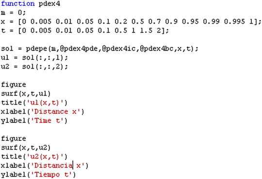
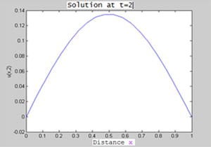
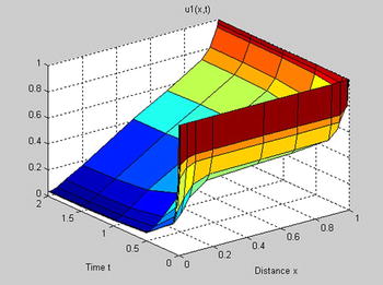
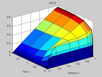
To view the solution (Figures 9-16 and 9-17), we enter the following in the MATLAB Command Window:
>> pdex4
EXERCISE 9-1
Solve the following Van der Pol system of equations:
We begin by defining a function named vdp100 in an M-file, where we will store the equations of the system. This function begins by defining a column vector with two empty rows which are subsequently assigned the components which make up the equation (Figure 9-18).
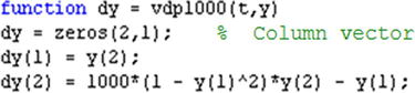
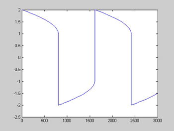
We then solve the system and plot the solution y1 = y1(t ) given by the first column (Figure 9-19) by typing the following into the Command Window:
>> [T, Y] = ode15s(@vdp1000,[0 3000],[2 0]);
>> plot(T, Y(:,1),'-')
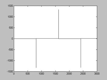
Similarly we plot the solution y2 = y2(t ) (Figure 9-20) by using the syntax:
>> plot(T, Y(:,2),'-')
EXERCISE 9-2
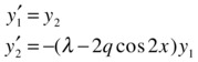
Given the following differential equation:
![]()
subject to the boundary conditions y (0) = 1, y '(0) = 0, y '(π) = 0, find a solution for q = 5 and λ = 15 based on an initial solution defined on 10 equally spaced points in the interval [0, π] and graph the first component of the solution on 100 equally spaced points in the interval [0, π].
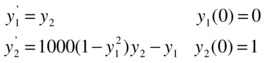
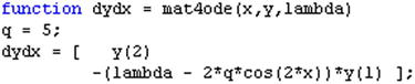
The given equation is equivalent to the following system of first order differential equations:
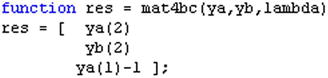
with the following boundary conditions:

The system of equations is introduced in the M-file shown in Figure 9-21, the boundary conditions are given in the M-file shown in Figure 9-22, and the M-file in Figure 9-23 sets up the initial solution.
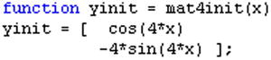
The initial solution for λ = 15 and 10 equally spaced points in [0,π ] is calculated using the following MATLAB syntax:
>> lambda = 15;
solinit = bvpinit(linspace(0,pi,10), @mat4init, lambda);
The numerical solution of the system is calculated using the following syntax:
>> sol = bvp4c(@mat4ode,@mat4bc,solinit);
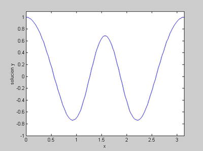
To graph the first component on 100 equally spaced points in the interval [0, π ] we use the following syntax:
>> xint = linspace(0,pi);
Sxint = bvpval(ground, xint);
plot(xint, Sxint(1,:)))
axis([0 pi-1 1.1])
xlabel('x')
ylabel('solution y')
The result is presented in Figure 9-24.
EXERCISE 9-3
Solve the following differential equation:
![]()
in the interval [0,20], taking as initial solution y = 2, y' = 0. Solve the more general equation
![]()
The general equation above is equivalent to the following system of first-order linear equations
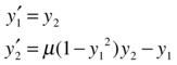
which is defined for μ = 1 in the M-file shown in Figure 9-25.
Taking the initial solution y1= 2 and y2= 0 in the interval [0,20], we can solve the system using the following MATLAB syntax:
>> [t, y] = ode45(@vdp1,[0 20],[2; 0])
t =
0
0.0000
0.0001
0.0001
0.0001
0.0002
0.0004
0.0005
0.0006
0.0012
.
.
19.9559
19.9780
20,0000
y =
2.0000 0
2.0000 - 0.0001
2.0000 - 0.0001
2.0000 - 0.0002
2.0000 - 0.0002
2.0000 - 0.0005
.
.
1.8729 1.0366
1.9358 0.7357
1.9787 0.4746
2.0046 0.2562
2.0096 0.1969
2.0133 0.1413
2.0158 0.0892
2.0172 0.0404
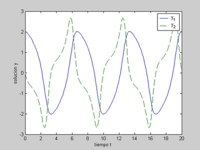
We can graph the solutions (Figure 9-26) by using the syntax:
>> plot(t, y(:,1),'-', t, y(:,2),'-')
>> xlabel('time t')
>> ylabel('solution y')
>> legend('y_1', 'y_2')
To solve the general system with the parameter μ, we define the system in the M-file shown in Figure 9-27.
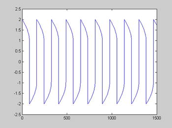
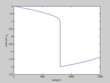
Now we can graph the first solution y1= 2 and y2= 0 corresponding to μ = 1000 in the interval [0,1500] using the following syntax (see Figure 9-28):
>> [t, y] = ode15s(@vdp2,[0 1500],[2; 0],[],1000);
>> xlabel('time t')
>> ylabel('solution y_1')
To graph the first solution y1 = 2 and y2 = 0 for another value of the parameter, for example μ = 100, in the interval [0,1500], we use the following syntax (see Figure 9-29):
>> [t, y] = ode15s(@vdp2,[0 1500],[2; 0],[],100);
>> plot(t, y(:,1),'-');