![]()
Functions
6.1 Custom Defined Functions
We already know that MATLAB has a wide variety of functions that can be used in everyday work with the program. But, in addition, MATLAB also offers the possibility of custom defined functions. The most common way to define a function is to write its definition to a text file, called an M-file, which will be permanent and will therefore enable the function to be used whenever required.
The second way to define a function is to use the relation between MATLAB and Maple, provided you have the symbolic math Toolbox installed. In this case, functions of a variable can also be directly defined.
6.2 Functions and M-files
MATLAB is usually used in command mode (or interactive mode), in which case a command is written in a single line in the Command Window and is immediately processed. But MATLAB also allows the implementation of sets of commands in batch mode, in which case a sequence of commands can be submitted which were previously written in a file. This file (M-file) must be stored on disk with the extension ".m" in the MATLAB subdirectory, using any ASCII editor or by selecting M-file New from the File menu in the top menu bar, which opens a text editor that will allow you to write command lines and save the file with a given name. Selecting M-File Open from the File menu in the top menu bar allows you to edit any pre-existing M-file.
To run an M-file simply type its name (without extension) in interactive mode into the Command Window and press Enter. MATLAB sequentially interprets all commands and statements of the M-file line by line and executes them. Normally the literal commands that MATLAB is performing do not appear on screen, except when the command echo on is active and only the results of successive executions of the interpreted commands are displayed. Work in batch mode is useful when automating large scale tedious processes which, if done manually, would be prone to mistakes. You can enter explanatory text and comments into M-files by starting each line of the comment with the symbol %. The help command can be used to display comments made in a particular M-file.
MATLAB provides certain commands which are frequently used in M-file scripts. Among them are the following:
echo on: View on-screen commands of an M-file script while it is running.

echo off: Hides on-screen commands of an M-file script (this is the default setting).

pause: Interrupts the execution of an M-file until the user presses a key to continue.

keyboard: Interrupts the execution of an M-file and passes the control to the keyboard so that the user can perform other tasks.  The execution of the M-file can be resumed by typing the return command into the Command Window and pressing Enter.

return: Resumes execution of an M-file after an outage.

break: Prematurely exits a loop.

clc: Clears the Command Window.

home: Hides the cursor.

more on: Enables paging of the MATLAB Command Window output.

more off: Disables paging of the MATLAB Command Window output.

more(N): Sets page size to N lines.

menu: Offers a choice between various types of menu for user input.
When you define a function using an M-file, the above commands can be used if necessary.
The command function allows you to define functions in MATLAB, making it one of the most useful applications of M-files. The syntax of this command is as follows:
function output_parameters = function_name (input_parameters)
the function body
Once the function has been defined, it is stored in an M-file for later use. It is also useful to enter some explanatory text in the syntax of the function (using %), which can be accessed later by using the help command.
When there is more than one output parameter, they are placed between square brackets and separated by commas. If there is more than one input parameter, they are separated by commas. The body of the function is the syntax that defines it, and should include commands or instructions that assign values to output parameters. Each command or instruction of the body often appears in a line that ends either with a comma or, when variables are being defined, by a semicolon (in order to avoid duplication of outputs when executing the function). The function is stored in the M-file named function_name.m.
Let us define the function fun1(x) = x ^ 3 - 2 x + cos(x), creating the corresponding M-file named fun1.m by using the syntax:
function p = fun1(x)
% Definition of a simple function
p = x ^ 3 - 2 * x + cos(x);
To define this function in MATLAB select M-file New from the File menu in the top menu bar (or click the button ![]() in the MATLAB tool bar). This opens the MATLAB Editor/Debugger text editor that will allow us to insert command lines defining the function, as shown in Figure 6-1.
in the MATLAB tool bar). This opens the MATLAB Editor/Debugger text editor that will allow us to insert command lines defining the function, as shown in Figure 6-1.

To permanently save this code in MATLAB select the Save option from the File menu at the top of the MATLAB Editor/Debugger. This opens the Save dialog of Figure 6-2, which we use to save our function with the desired name and in the subdirectory indicated as a path in the file name field. Alternatively you can click on the button ![]() or select Save and run from the Debug menu. Functions should be saved using a file name equal to the name of the function and in MATLAB’s default work subdirectory C: MATLAB6p1work.
or select Save and run from the Debug menu. Functions should be saved using a file name equal to the name of the function and in MATLAB’s default work subdirectory C: MATLAB6p1work.

Once a function has been defined and saved in an M-file, it can be used from the Command Window. For example, to find the value of the function at 3π-2 we write in the Command Window:
>> fun1(pi)

ans =

   23.7231
For help on the previous function (assuming that comments were added to the M-file that defines it) you use the command help, as follows:
>> help fun1(x)

 A simple function definition
The definition of a function with more than one input parameter and more than one output parameter is illustrated in the following example (Figure 6-3):
function [x1,x2]=equation2(a,b,c)
% This function solves the quadratic equation ax ^ 2 + bx + c = 0
% whose coefficients are a, b and c (input parameters)
% and whose solutions are x 1 and x 2 (output parameters)
d=b^2-4*a*c;
x1=(-b+sqrt(d))/(2*a);
x 2 = (-b-sqrt (d)) /(2*a);

The saved M-file with the name equation2.m will solve the equation x ^ 2-6 x + 2 = 0 in the following way:
>> [p,q]=equation2(1,-6,2)

p =

    5.6458

q =

    0.3542
We can also ask for help about the function equation2.
>> help equation2

  This function solves the quadratic equation ax ^ 2 + bx + c = 0
  whose coefficients are a, b and c (input parameters)
  and whose solutions are x1 and x2 (output parameters)
We can also evaluate a function defined in an M-file using the command feval, whose syntax is as follows:
feval('F', arg1, arg1,..., argn) evaluates the function F (M-file F.m) with the specified arguments arg1 arg2,..., argn
For example, we can evaluate previously defined functions using the command feval:
>> [r1,r2]=feval('equation2',1,-6,2)

r1 =

    5.6458

R2 =

    0.3542

>> feval('fun1',pi)

ans =

   23.7231
6.3 Functions and Flow Control. Loops
The use of recursive functions, conditional operations and piecewise defined functions is very common in mathematics. The handling of loops is necessary for the definition of these types of functions. Naturally, the definition of the functions will be made via M-files or through the relationship with Maple, via the symbolic math Toolbox.
6.4 The FOR loop
MATLAB has its own version of the DO statement (defined in the syntax of most programming languages). This statement allows you to run a command or group of commands repeatedly. For example:
>> for i=1:3, x(i)=0, end

x =

     0

x =

     0     0

x =

     0 0 0
The general form of a FOR loop is as follows:
for variable = expression
       commands
end
The loop always starts with the clause for and ends with the clause end, and includes in its interior a whole set of commands that are separated by commas. If any command defines a variable, it must end with a semicolon in order to avoid repetition in the output. Typically, loops are used in the syntax of M-files. Here is an example:
for i=1:m,
    for j=1:n,
        A(i,j)=1/(i+j-1);
    end
end
In this loop (Figure 6-4) we have defined the Hilbert matrix of order (m, n). If we save the M-file (Figure 6-5) as for1.m, we can build any Hilbert matrix by running the M-file and specifying values for the variables m and n as shown below:
>> m = 3, n = 4; for1; A

A =

    1.0000    0.5000    0.3333    0.2500
    0.5000    0.3333    0.2500    0.2000
    0.3333    0.2500    0.2000    0.1667


6.5 The WHILE loop
MATLAB has its own version of the WHILE structure defined in the syntax of most programming languages. This statement allows you to repeat a command or group of commands a number of times while a specified logical condition is met. The general syntax of this loop is as follows:
While condition
commands
end
The loop always starts with the clause while, followed by a condition, and ends with the clause end, and includes in its interior a whole set of commands that are separated by commas which continually loop while the condition is met. If any command defines a variable, it must end with a semicolon in order to avoid repetition in the output. As an example, we write an M-file that is saved as while1.m, which calculates the largest number whose factorial does not exceed 10100.
n=1;
while prod(1:n) < 1.e100,
      n = n + 1;
end,
n
Now, we run the M-file:
>> while1

n =

    70
6.6 IF ELSEIF ELSE END LOOP
MATLAB, like most structured programming languages, also includes the IF-ELSEIF-ELSE-END structure. Using this structure, scripts can be run if certain conditions are met. The loop syntax is as follows:
If condition
   commands
end
In this case the commands are executed if the condition is true. But the syntax of this loop may be more general.
If condition
   commands1
else
   commands2
end
In this case, the commands1 are executed if the condition is true, and the commands2 are executed if the condition is false.
The IF statements, as well as FOR statements, can be nested. When multiple IF statements are nested, use the ELSEIF statement, whose general syntax is as follows:
if condition1
   commands1
ElseIf condition2
   commands2
ElseIf condition3
   commands3
.
.
else
end
In this case, the commands1 are executed if condition1 is true, the commands2 are executed if condition1 is false and condition2 is true, the commands3 are executed if condition1 and condition2 are false and condition3 is true, and so on.
The previous nested syntax is equivalent to the following unnested syntax, but executes much faster:
if condition1
   commands1
else
      If condition2
         commands2
     else
           if condition3
              commands3
          else
.
.
         end
     end
end
Consider as an example the following M-file named else1.m:
If n < 0,
   A = 'n is negative'
elseif rem(n,2) ==0
   A = 'n is even'
else
   A = 'n is odd'
end
Running it, we obtain the number type (negative, odd or even) for a specified value of n:
>> n = 8; else1

A =

n is even

>> n = 7; else1

A =

n is odd

>> n =-2; else1

A =

n is negative
6.7 Recursive Functions
One of the applications of loops is the creation of recursive functions via M-files. For example, although the factorial function can be defined in MATLAB as n! = prod(1:n), it can be also defined as a recursive function in the following way:
function y=factori(x)
       if x==0
        y=1;
       end
       if x==1
        y=1;
       end
       if x>1
        y=x*feval('factori',x-1);
      end
If we now want to calculate 40!, we do the following:
>> factori(40)

ans =

  8. 1592e + 047
EXERCISE 6-1
The Fibonacci sequence {an} is defined by the recurrence law a1 = 1, a2 = 1, an = an-1 + an-2. Represent this succession by a recurrent function and calculate a2 , a5 and a20.
We define the function using the M-file fibo.m as follows:
function y=fibo(x)
if x<=1
y = 1;
else y = feval('fibo',x-1) + feval('fibo',x-2);
end
>> fibo(2)
ans =
2
>> fibo(5)
ans =
8
>> fibo(20)
ans =
10946
EXERCISE 6-2
Newton’s method for solving the equation f (x) = 0, under certain conditions on f, is via the iteration xr+1 = xr - f(xr )/f ’(xr ) for an initial value x0 sufficiently close to a solution. Write a program that solves equations by Newton’s method to a given precision and use it to calculate the root of the equation x3 - 10 x2 + 29 x - 20 = 0 close to the point x = 7 with an accuracy of 0.00005. Also search for a solution setting the precision to 0.0005.
The program code would read as follows:
% x is the initial value, precis is the precision required
% func is the function f and dfunc is its derivative
it=0; x0=x;
d=feval(func,x0)/feval(dfunc,x0);
while abs(d)>precis
x1=x0-d;
it=it+1;
x0=x1;
d=feval(func,x0)/feval(dfunc,x0);
end;
res = x0;
We save the program in the file named fnewton.m.
Now, we define the function f (x) = x3 - 10 x2 x + 29 - 20 and its derivative via the M-files named f302.m and f303.m in the following way:
F=x.^3-10.0*x.^2+29.0*x-20.0;
function F=f303(x);
F=3*x.^2-20*x+29;
To run the program that solves the given equation we type:
>> [x, it]=fnewton('f302','f303',7,.00005)
x =
5.000
it =
6
After 6 iterations and with an accuracy of 0.00005 we have obtained the solution x = 5. For 5 iterations and a precision of 0.0005 we get x = 5.0002 via:
>> [x, it] = fnewton('f302','f303',7,.0005)
x =
5.0002
it =
5
EXERCISE 6-3
Schröder’s method, which is similar to Newton’s method for solving the equation f (x) = 0, under certain conditions required on f, uses the iteration x = xr+1 = xr -m f(xr )/f’(xr ) for a given initial value x0 close enough to a solution, m being the order of multiplicity of the sought root. Write a program that solves equations using Schröder’s method to a given precision and use it to calculate a root with multiplicity 2 of the equation (e -x -x)2 = 0 close to the point x =-2 to an accuracy of 0.00005.
The program code reads as follows:
% m is the order of the multiplicity of the root
% x is the initial value, precis is precision
it=0; x0=x;
d=feval(func,x0)/feval(dfunc,x0);
while abs(d)>precis
x1=x0-m*d;
it=it+1; x0=x1;
d=feval(func,x0)/feval(dfunc,x0);
end;
res = x 0;
We save the program in the file named schroder.m.
Now, we define the function f (x) = (e -x -x)2 and its derivative and save them in files named f304.m and f305.m:
function F=f304(x);
F=(exp(-x)-x).^2;
function F=f305(x);
F=2.0*(exp(-x)-x).*(-exp(-x)-1);
To run the program that solves the stated equation type:
>>[x,it]=schroder('f304','f305',2,-2,.00005)
x =
0.5671
it =
5
In 5 iterations we obtain the solution x = 0.56715.
6.8 Conditional Functions
Functions defined differently on different intervals of variation in the independent variable have always played an important role in mathematics. MATLAB enables you to work with these types of functions, which are usually defined using M-files, in the majority of cases relying on FOR loops, WHILE loops, IF-ELSEIF-IF-END, etc.
EXERCISE 6-4
Define the function delta (x), which has value 1 if x = 0, and 0 if x is non-zero. Also define the function delta1 (x), which has the value 0 if x = 0, 1 if x > 0, and - 1 if x < 0, and represent it graphically.
Define delta (x) by creating the M-file delta.m as follows:
function y = delta (x)
If x == 0
y = 1;
else y = 0;
end
To define delta1(x) we create the M-file delta1.m as follows:
function y = delta1 (x)
If x == 0
y = 0;
ElseIf x > 0 and = 1;
ElseIf x < 0 and =-1;
end
To graph a function, we use the command fplot, whose syntax is as follows:
fplot [xmin xmax ymin ymax] ('function')
This represents the function in the given ranges of x and y.
Now, we represent the function delta1 (x). See Figure 6-6:
>> fplot ('delta1(x)', [-10 10 -2 2])

EXERCISE 6-5
Define a function stat (v) which returns the mean and standard deviation of the elements of a given vector v. As an application, find the mean and standard deviation of the numbers 1, 5, 6, 7 and 9.
To define stat (v), we create the M-file stat.m as follows:
function [media, destip] = stat(v)
[m,n]=size(v);
if m==1
m=n;
end
media=sum(v)/m;
destip=sqrt(sum(v.^2)/m-media.^2);
Now we calculate the mean and standard deviation of the numbers 1, 5, 6, 7 and 9:
>> [a,s]=stat([1 5 6 7 9])
a =
5.6000
s =
2.6533
EXERCISE 6-6
Define and graph the piecewise function that has the value 0 if x≤ -3, x3 if -3<x<-2, x2 if -2≤x≤2, x if 2<x<3 and 0 if 3≤x.
We create the function using an M-file named piece1.m:
function y=piece1(x)
if x<=-3
y = 0;
ElseIf - 3 < x & x < - 2
y = x ^ 3;
ElseIf - 2 < = x & x < = 2
y = x ^ 2;
elseif 2<x & x<3
y=x
elseif x>=3
y = 0;
end
Now, we graph the function (see Figure 6-7):
>> fplot('piece1', [-5 5])

6.9 Defining Functions Directly. Evaluating Functions
We already know that we can define and evaluate functions by making use of the relation between MATLAB and Maple, provided the symbolic mathematics Toolbox is available. Using this tool, you can define functions of one or severable variables using the command maple.
The advantage of defining functions in this way is that it is not necessary to write files to disk.
6.10 Functions of One Variable
Functions of one variable are defined in the form f = 'function' (or f = function whenever its variables have previously been defined as symbolic with syms).
To find the value of the function f at a point, you use the command subs, whose syntax is as follows:
subs(f,a) applies the function f at the point a

subs(f,a,b) substitutes in f the value b by the value a
Let's see how to define the function f (x) = x ^ 2 :
>> f='x^2'  (or: syms x, f = x ^ 2)

f =

x ^ 2
Now we calculate the values f (4), f (a+1) and f(3x+x^2):
>> A=subs(f,4),B=subs(f,'a+1'),C=subs(f,'(3*x+x^2)')

A =

16

B =

(a+1) ^ 2

C =

(3 * x + x ^ 2) ^ 2
6.11 Functions of Several Variables
Functions of one or several variables are defined using the maple command as follows:
maple('f: = x - > f (x)') defines the function f(x)

maple('f:=(x,y,z,...)- > f(x,y,z,...)') defines the function f(x,y,z,...)

maple('f:=(x,y,z,...)- > (f1(x,y,...), f2(x,y,...),...)') defines the vector function (f1(x,y,...), f2(x,y,...),...)
To find the value of the function (x, y, z) - > f(x,y,z...) at the point (a, b, c,...) the expression maple ('f(a,b,c,...)') is used.
The value of the vector function f:=(x,y,...)-> (f1(x,y,...), f2(x,y,...),...) at the point (a, b,...) is found using the expression maple ('f(a,b,...)').
The function f(x,y) = 2x + y is defined in the following way:
>> maple('f:=(x,y) - > 2 * x + y');
f (2,3) and f(a,b) are calculated as follows:
>> maple('f(2,3)')

ans =

7

>> maple('f(a,b)')

ans =

2 * a + b
EXERCISE 6-7
Define the functions f (x) = x2 , g (x) = x1/2 and h (x) = x + sin (x). Calculate f (2), g(4) and h(a-b2).
>> f ='x ^ 2', g = 'x ^(1/2)', h = 'x+sin(x)'
f =
x ^ 2
g =
x ^(1/2)
h =
x+sin (x)
>> a=subs(f,2),b=subs(g,4),c=subs(h,'a-b^2')
a =
4
b =
4 ^(1/2)
c =
a-b ^ 2 + sin(a-b^2)
EXERCISE 6-8
Given the function h defined by h(x,y) = (cos(x2-y2), sin(x2-y2)), calculate h (1,2), h(-pi,pi) and h(cos (a2), cos (1 -a2)).
As it is a vector function of two variables, we use the command maple:
>> maple('h:=(x,y) - > (cos(x^2-y^2), sin(x^2-y^2))');
>> maple('A = h (1, 2), B = h(-pi,pi), C = h(cos(a^2), cos(1-a^2))')
ans =
A = (cos (3),-sin (3)), B = (1, 0),
C = (cos (cos(a^2) ^ 2-cos(-1+a^2) ^ 2), sin(cos(a^2) ^ 2-cos(-1+a^2) ^ 2))
We could also define this vector function of two variables using the M-file named vector1.m below:
function [z,t] = vector1(x,y)
z = cos(x^2-y^2);
t = sin(x^2-y^2);
You can also build the function with the following syntax:
function h = vector1(x,y)
z = cos(x^2-y^2);
t = sin(x^2-y^2);
h = [z,t];
We calculate the values of the function at (1,2) and (-pi, pi) as follows:
>> A = vector1(1,2), B = vector1(-pi,pi)
A =
-0.9900 - 0.1411
B =
1 0
EXERCISE 6-9
Given the function f defined by:
f(x,y)= 3(1-x)2 e -(y+1)^2-x^2 -10(x/5-x 3-y/5)e -x^2-y^2-1/3e -(x+1)^2-y^2
find f (0,0) and represent it graphically.
First, we can define it via the maple command:
>> maple ('f:=(x,y) - > 3 *(1-x) ^ 2 * exp (-(y + 1) ^ 2-x ^ 2)-
10*(x/5-x^3-y^5)*exp(-x^2-y^2)-1/3*exp(-(x+1)^2-y^2)');
Now, we calculate the value of f at (0,0):
>> maple('f(0,0)')
ans =
8/3*exp(-1)
We can also create the M-file named func2.m as follows:
function h = func2(x,y)
h=3*(1-x)^2*exp(-(y+1)^2-x^2)-10*(x/5-x^3-y^5)*exp(-x^2-y^2)-
1/3 * exp (-(x + 1) ^ 2 - y ^ 2);
Now, we calculate the value of h at (0,0):
>> func2(0,0)
ans =
0.9810
To graph the function, we use the command meshgrid to define the x and y ranges for the domain of the function (a neighborhood of the origin) and the command surfing to graph the surface:
>> [x,y] = meshgrid(-0.1:.005:0.1,-0.1:.005:0.1);
>> z = func2(x,y);
>> surf(x,y,z)
This yields the graph shown in Figure 6-8:

6.12 Piecewise Functions
MATLAB provides a direct command that enables you to define conditional functions that take different values depending on different intervals of definition of the variables (piecewise functions). The command in question is piecewise, and its syntax is presented below:
maple ('piecewise(expr1, value1, expr2, value2,..., exprn, valuen)')
- Defines the piecewise function that takes value1 if the variable satisfies expr1, takes value2 if the variable satisfies expr2, and so on. For all values of the function not covered by the expressions the function takes the value zero.
maple ('piecewise(expr1, value1, expr2, value2,..., exprn, valuen, valuem)')
- Defines the piecewise function that takes value1 if the variable satisfies expr1, takes value2 if the variable satisfies expr2, and so on. For all values of the function not covered by the expressions the function takes the value valuem.
maple ('convert (expression,piecewise)')
- Converts the expression containing Heavside, abs, signum, etc. functions to a piecewise function. The command can be applied to a list or set of expressions which is converted to a list or set.
maple ('convert (expression, piecewise variable)')
- Converts the expression containing Heavside, abs, signum, etc. functions to a piecewise function according to the specified variable.
maple ('convert (expression,pwlist)')
- Converts the expression containing functions to its representation in the form of a piecewise list.
maple ('convert (expression, pwlist,variable)')
- Converts the expression containing functions to its representation in the form of a piecewise list based on the specified variable.
A great advantage of this command is that it can be used together with commands like discont, diff, int, dsolve. This allows you to directly analyze the continuity, differentiability and integrability of piecewise-defined functions. At the same time, it allows this type of function to be used in the analysis of differential equations. Here are some examples:
>> pretty(sym(maple('piecewise(x>0,x)')))

                         |x           0 < x

                         | 0        otherwise

>> pretty(sym(maple('piecewise(x*x>4 and x<8,f(x))')))

                                           2
                | f (x)             4 - x < 0 and x - 8 < 0

                |  0                 otherwise

>> pretty(sym(maple('simplify(piecewise(x*x>4 and x<8,f(x)))')))

                         | f (x)       x < - 2
                         |
                         |  0          x < = 2

                         | f(x)        x < 8
                         |
                         |  0          8 <= x

>> pretty(sym(maple('piecewise(x<0,-1,x<1,0,1)')))

                        | -1      x < 0
                        |
                        0      x < 1
                        |
                        | 1      otherwise
It is possible to define piecewise functions using the arrow operator, and to evaluate previously defined functions at different points.
>> pretty(sym(maple('f:=x->piecewise(x<0,-1,x<1,0,1) : f(1/2)')))

                                  0

>> pretty(sym(maple('f(5),f(-5),f(-infinity),f(infinity)')))

                             1, - 1, - 1, 1
You can also directly simplify functions defined in terms of predefined piecewise functions
>> pretty(sym(maple('p:= piecewise(x<0,-x,x>0,x):p'))

                                 | -x        x < 0
                        p:=
                                 | x         0 < x

>> pretty(sym(maple('p:= piecewise(x<0,-x,x>0,x):simplify(p^2 + 5)')))

                                 2
                                x + 5
However, you cannot directly simplify functions defined in terms of predefined piecewise functions that include parameters.
>> pretty(sym(maple('p:= piecewise(x<a,x,x>b,x*x):p')))

                                | x         x < a
                                |
                        p:=
                                |   2
                                | x         b < x

>> pretty(sym(maple('p:= piecewise(x<a,x,x>b,x*x):simplify(p^2)')))

                         | x         x < a^ 2
                         |

                         |   2
                         | x         b < x
To simplify the above expression, we need to convert it into a piecewise function in terms of the main variable x.
>>  pretty(sym(maple('convert(p,piecewise,x)')))

                          |   2
                          | x             x < a
                          |
                            0             x = a
                          |
                          |   4
                          | x             a < x
A piecewise function can also be expressed as a list.
>> pretty(sym(maple('f:=piecewise(x<0,-1,x<1,0,1):')));
>> pretty(sym(maple('convert(f,pwlist)')))

                           [- 1, 0, 0, 1, 1]
EXERCISE 6-10
Given the function f of a real variable defined by:
f(x)= |(1-|x|) |
express it as a piecewise-defined function and represent it graphically.
>> pretty(sym(maple('convert(abs(1-abs(x)),piecewise)')))
| -1 - x x <= -1
|
| x + 1 x <= 0
![]()
| 1 - x x < 1
|
| x - 1 1 <= x
Below, we represent the piecewise function using the ezplot command (see Figure 6-9) which can be used for general representations of functions of one variable.
>> ezplot('abs(1-abs(x))',[-2,2])

EXERCISE 6-11
Given the function p of a real variable defined by:
p (x) =-1 if x < 0, p (x) = 2 x if x > 1 and p (x) = x2 otherwise
express it as a piecewise-defined function. Find its indefinite integral and its derivative.
>> pretty(sym(maple('p:=piecewise(x<0, -1, x>1, 2*x, x^2):p')))
| -1 x < 0
|
p:= ![]() 2 x 1 < x
2 x 1 < x
|
| 2
| x otherwise
Now, let’s calculate the indefinite integral of the function p (x).
>> pretty(sym(maple('h:=int(p,x):h')))
| -x x < = 0
|
| 3
h:= ![]() 1/3 x x <= 1
1/3 x x <= 1
|
| 2
| x - 2/3 1 < x
Next, we find the first derivative of p (x):
>> pretty(sym(maple('d:=diff(p,x):d')))
| 0 x <= 0
|
| 2 x x <= 1
|
d:= ![]() 2 1 < x
2 1 < x
|
| undefined x = 1
|
| undefined x = 0
Note that the function p (x) is not differentiable at the points x = 1 and x = 0.
EXERCISE 6-12
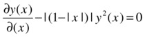
Given the function of a real variable p defined in the previous exercise, solve the following differential equation:

>> maple('dsolve(diff(y(x), x) + p * y(x) = 0, y(x))');
>> pretty(sym(maple('dsolve(diff(y(x), x) + p * y(x) = 0, y(x))')))
| _C1 exp (x) x < = 0
|
| 3
y (x) = ![]() _C1 exp(-1/3 x) x < = 1
_C1 exp(-1/3 x) x < = 1
|
| 2
| _C1 exp(-x + 2/3) 1 < x
EXERCISE 6-13
Solve the following differential equation:
>> pretty(sym(maple('convert(abs(1-abs(x)),piecewise)')))
| -1 - x x <= -1
|
| 1 + x x <= 0
![]()
| 1 - x x <= 1
|
| x - 1 1 < x
>> pretty(sym(maple('dsolve(diff(y(x),x)=convert(abs(1-abs(x)),piecewise)* y(x)^2,y(x))')))
| 2
| - ----------------- x <= -1
| 2
| -2 x - x + 2 _C1
|
| 2
| - -------------------- x <= 0
| 2
| 2 x + 2 + x + 2 _C1
y(x) = ![]()
| 2
| - -------------------- x <= 1
| 2
| 2 x + 2 - x + 2 _C1
|
| 2
| - --------------------- 1 < x
| 2
| -2 x + 4 + x + 2 _C1
6.13 Functional Operations
Normally, functions defined in MATLAB operate on their arguments. However, there are also functional operators that operate on other functions (i.e. functional operators have functions as arguments), for example, the inverse function operator. MATLAB also allows the classical operations between functions (sum, product, etc.).
Among the functional operators and classical operations between functions offered by MATLAB, we highlight the following:
syms x y z...

f = f(x,y,z,...), g = g(x,y,z,...), h = h(x,y,z,...)...

symadd(f,g) adds the functions f and g (i.e. f + g)

symop(f,'+',g,'+',h,'+',...) performs the sum f+g+h+...

maple('f+g+h+...') performs the sum  f+g+h +...

symsub(f,g) subtracts g from f (i.e. f-g)

symop(f,'-',g,'-',h,'-',...) forms the successive difference f-g-h-...

maple('f-g-h-...)') forms the successive difference f-g-h-...

symmul(f, g) finds the product of f and g (i.e. f * g)

symop(f,' * ',g,' * ',h,' * ',...) forms the product  f*g*h*...

maple('f*g*h*,...) ') forms the product f * g * h *...

symdiv(f,g) finds the quotient f / g

symop(f,'/',g,'/ ',h,'/ ',...) forms the successive quotient f/(g/(h/...

maple('f/g/h/...) ') forms the successive quotient f/(g/(h/...

sympow(f,k) raises f to the power k (k is a scalar)

symop(f,'^',g) raises a function f to the power of another function g

maple('f^g') raises a function f to the power of another function g

compose(f,g) composes two functions f and g (i.e. f(g(x)))

compose(f,g,u) composes the functions f and g, taking the expression u as the domain of f and g

maple('f @g @h @...') composes the functions f, g, h...

maple('f(g(h(...)'))) composes the functions f, g, h...

g = finverse(f) gives the inverse of the function f

g = finverse(f,v) gives the inverse of the function f using the symbolic variable v as an independent variable

maple('invfunc[f(x)]') gives the inverse of the function f(x)

maple('f(x)@@(-1)') gives the inverse of the function f(x)

maple('map(function,exp)') applies the given function to each operand or element of the expression (according to the first level of operations), where exp is a list or set

maple('map2(f,exp,list)') applies the function f to the elements of the list, in such a way that the function has as its first argument the constant expression expr, and as the second argument, each item in the specified list

maple('unapply(expr,x1,x2,...,xn)') returns an operator from the expression expr in the variables x1, x2,..., xn

maple('applyop(f,n,expr)') applies the function to the nth operand of the expression

maple('applyop(function,{n1, n2,..., nk},expr)') applies the function to the n1, n2,..., nk-th operands of the expression

maple('applyop(function,n,expr,arg2,..., argn)') replaces the nth operand of the expression expr by the result of applying the given function to it, passing arg2,..., argn as additional arguments
Here are some examples:
>> maple('p: = x ^ 2 + sin (x) + 1')

ans =

p := x^2+sin(x)+1

>>  pretty(sym(maple('f:= unapply(p,x):f')))

                                   2
                             x -> x  + sin(x) + 1

>> pretty(sym(maple('f(Pi/6)')))

                                    2
                             1/36 pi + 3/2

>> maple('q:= x^2 + y^3 + 1'):
>> pretty(sym(maple('f:= unapply(q,x) :f')))


                                   2    3
                             x -> x  + y  + 1

>> pretty(sym(maple('f(2)')))

                                     3
                                5 + y

>> pretty(sym(maple('g:= unapply(q,x,y) :g')))


                                       2    3
                            (x, y) -> x  + y  + 1

>> pretty(sym(maple('g(2,3)')))

                                  32
>> clear all
>> maple('p:= y^2-2*y-3');
>> pretty(sym(maple('applyop(f,2,p)')))

                            2
                           y  + f(-2 y) - 3

>> pretty(sym(maple('applyop(f,2,p,x1,x2)')))


                        2
                       y  + f(-2 y, x1, x2) - 3

>> pretty(sym(maple('applyop(f,{2,3},p)')))


                          2
                         y + f(-2 y) + f (- 3)

>> pretty(sym(maple('map(f,x + y*z)')))

                            f (x) + f(y z)

>> pretty(sym(maple('map(f,{a,b,c})')))

                          {f(a), f(b), f(c)}

>> pretty(sym(maple('map(x -> x^2, x + y)')))

                                2    2
                               x  + y

>> pretty(sym(maple('map2(f,g,{a,b,c})')))

                     {f(g, a), f(g, b), f(g, c)}

>> pretty(sym(maple('map(diff,[(x+1)*(x+2),x*(x+2)],x)')))

                          [2 x + 3, 2 x + 2]

>> pretty(sym(maple('map2(diff,x^y/z,[x,y,z])')))

                         y     y            y
                        x y   x  ln(x)     x
                       [----, --------, - ----]
                        x z      z          2
                                           z
EXERCISE 6-14
Let f(x) = x2+ x, g(x) = x3+ 1 and h(x) = sin (x) + cos (x). Calculate:
f (g(x)), g(f(x-1)), f(h(Pi/3)) and f(g(h(sinx))).
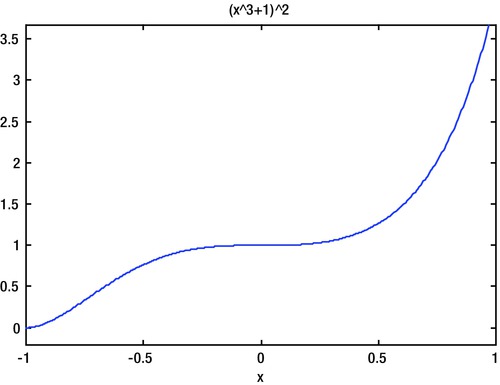
Graph f(g(x)) on the interval [- 1,1].
>> syms x
>> f = x ^ 2; g = x ^ 3 + 1; h = sin (x) + cos (x); u = compose(f, g)
u =
(x ^ 3 + 1) ^ 2
>> v = subs(compose(g,f),x-1)
v =
(x-1)^6+1
>> w=subs(compose(f,h),'pi/3')
w =
(sin(1/3*pi) + cos(1/3*pi)) ^ 2
>> r = subs(compose(f,compose(g, h)), sin (x))
r =
((sin (sin (x)) + cos (sin (x))) ^ 3 + 1) ^ 2
This can also be solved in the following way:
>> maple('f: = x - > x ^ 2; g: = x - > x ^ 3 + 1, h: = x - > sin(x) + cos(x)');
>> maple('(f(g(h(sin(x)))')))
ans =
((sin(sin (x)) + cos (sin (x))) ^ 3 + 1) ^ 2
To graph the function f (g (x)) we use the command ezplot, which, like fplot, graphs functions of a single variable as follows (see Figure 6-10):
>> ezplot(subs(compose(f,g),x),[-1,1])
EXERCISE 6-15
Define the functions f and g by f(x,y) =(x2,y2) and g(x,y) = (sin(x), sin(y)). Calculate f (f (f(x,y))) and g(f(π,π)).
>> maple('f:=(x,y) - >(x^2,y^2); g:=(x,y) - > (sin(x), cos(y))');
>> a = maple('(f(f(f(x,y)))'))
a =
x ^ 8, y ^ 8
>> maple('(g(f(pi,pi)))')
ans =
sin(pi^2), cos(pi^2)
EXERCISE 6-16
Calculate the inverse of each of the functions f (x) = sin (cos (x1/2) and g (x) = sqrt (tan (x2)).
>> syms x, f = (cos(x ^(1/2)));
>> finverse(f)
ans =
arccos(arcsin(x))^2
>> g=sqrt(tan(x^2));
>> finverse(g)
Warning: finverse(sqrt(tan(x^2))) is not unique
ans =
arctan(x^2) ^(1/2)
In the latter case the program warns us of the non-uniqueness of the inverse function.