![]()
Programming and Numerical Analysis
7.1 MATLAB and Programming
MATLAB can be used as a high-level programming language including data structures, functions, instructions for flow control, management of inputs/outputs and even object-oriented programming. MATLAB programs are usually written into files called M-files. An M-file is nothing more than a MATLAB code (script) that executes a series of commands or functions that accept arguments and produces an output. The M-files are created using the text editor.
7.2 The Text Editor
The Editor/Debugger is activated by clicking on the create a new M-file button ![]() in the MATLAB desktop or by selecting File
in the MATLAB desktop or by selecting File ![]() New
New ![]() M-file in the MATLAB desktop (Figure 7-1) or Command Window (Figure 7-2). The Editor/Debugger opens a file in which we create the M-file, i.e. a blank file into which we will write MATLAB programming code (Figure 7-3). You can open an existing M-file using File
M-file in the MATLAB desktop (Figure 7-1) or Command Window (Figure 7-2). The Editor/Debugger opens a file in which we create the M-file, i.e. a blank file into which we will write MATLAB programming code (Figure 7-3). You can open an existing M-file using File ![]() Open on the MATLAB desktop (Figure 7-1) or, alternatively, you can use the command Open in the Command Window (Figure 7-2). You can also open the Editor/Debugger by right-clicking on the Current Directory window and choosing New
Open on the MATLAB desktop (Figure 7-1) or, alternatively, you can use the command Open in the Command Window (Figure 7-2). You can also open the Editor/Debugger by right-clicking on the Current Directory window and choosing New ![]() M-file from the resulting pop-up menu (Figure 7-4). Using the menu option Open, you can open an existing M-file. You can open several M-files simultaneously, each of which will appear in a different window.
M-file from the resulting pop-up menu (Figure 7-4). Using the menu option Open, you can open an existing M-file. You can open several M-files simultaneously, each of which will appear in a different window.


Figure 7-5 shows the functions of the icons in the Editor/Debugger.

7.3 Scripts
Scripts are the simplest possible M-files. A script has no input or output arguments. It simply consists of instructions that MATLAB executes sequentially and that could also be submitted in a sequence in the Command Window. Scripts operate with existing data on the workspace or new data created by the script. Any variable that is used by a script will remain in the workspace and can be used in further calculations after the end of the script.
Below is an example of a script that generates several curves in polar form, representing flower petals. Once the syntax of the script has been entered into the editor (Figure 7-6), it is stored in the work library (work) and simultaneously executes by clicking the button ![]() or by selecting the option Save and run from the Debug menu (or pressing F5). To move from one chart to the next press ENTER.
or by selecting the option Save and run from the Debug menu (or pressing F5). To move from one chart to the next press ENTER.


7.4 Functions and M-files. Eval and feval
We already know that MATLAB has a wide variety of functions that can be used in everyday work with the program. But, in addition, the program also offers the possibility of custom defined functions. The most common way to define a function is to write its definition to a text file, called an M-file, which will be permanent and will therefore enable the function to be used whenever required.
MATLAB is usually used in command mode (or interactive mode), in which case a command is written in a single line in the Command Window and is immediately processed. But MATLAB also allows the implementation of sets of commands in batch mode, in which case a sequence of commands can be submitted which were previously written in a file. This file (M-file) must be stored on disk with the extension ".m" in the MATLAB subdirectory, using any ASCII editor or by selecting M-file New from the File menu in the top menu bar, which opens a text editor that will allow you to write command lines and save the file with a given name. Selecting M-File Open from the File menu in the top menu bar allows you to edit any pre-existing M-file.
To run an M-file simply type its name (without extension) in interactive mode into the Command Window and press Enter. MATLAB sequentially interprets all commands and statements of the M-file line by line and executes them. Normally the literal commands that MATLAB is performing do not appear on screen, except when the command echo on is active and only the results of successive executions of the interpreted commands are displayed. Normally, work in batch mode is useful when automating large scale tedious processes which, if done manually, would be prone to mistakes. You can enter explanatory text and comments into M-files by starting each line of the comment with the symbol %. The help command can be used to display comments made in a particular M-file.
The command function allows the definition of functions in MATLAB, making it one of the most useful applications of M-files. The syntax of this command is as follows:
function output_parameters = function_name (input_parameters)
the function body
Once the function has been defined, it is stored in an M-file for later use. It is also useful to enter some explanatory text in the syntax of the function (using %), which can be accessed later by using the help command.
When there is more than one output parameter, they are placed between square brackets and separated by commas. If there is more than one input parameter, they are separated by commas. The body of the function is the syntax that defines it, and should include commands or instructions that assign values to output parameters. Each command or instruction of the body often appears in a line that ends either with a comma or, when variables are being defined, by a semicolon (in order to avoid duplication of outputs when executing the function). The function is stored in the M-file named function_name.m.
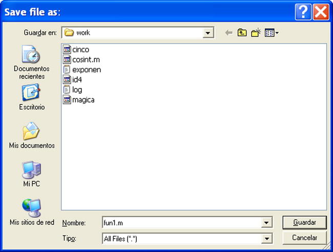
Let us define the function fun1(x) = x ^ 3 - 2 x + cos(x), creating the corresponding M-file fun1.m. To define this function in MATLAB select M-file New from the File menu in the top menu bar (or click the button ![]() in the MATLAB tool bar). This opens the MATLAB Editor/Debugger text editor that will allow us to insert command lines defining the function, as shown in Figure 7-11.
in the MATLAB tool bar). This opens the MATLAB Editor/Debugger text editor that will allow us to insert command lines defining the function, as shown in Figure 7-11.

To permanently save this code in MATLAB select the Save option from the File menu at the top of the MATLAB Editor/Debugger. This opens the Save dialog of Figure 7-12, which we use to save our function with the desired name and in the subdirectory indicated as a path in the file name field. Alternatively you can click on the button ![]() or select Save and run from the Debug menu. Functions should be saved using a file name equal to the name of the function and in MATLAB’s default work subdirectory C: MATLAB6p1work.
or select Save and run from the Debug menu. Functions should be saved using a file name equal to the name of the function and in MATLAB’s default work subdirectory C: MATLAB6p1work.
Once a function has been defined and saved in an M-file, it can be used from the Command Window. For example, to find the value of the function at 3π-2 we write in the Command Window:
>> fun1(3*pi/2)
ans =
95.2214
For help on the previous function (assuming that comments were added to the M-file that defines it) you use the command help, as follows:
>> help fun1(x)
7.4.1 A Simple Function Definition
A function can also be evaluated at some given arguments (input parameters) via the feval command, the syntax of which is as follows:
feval ('F', arg1, arg1,..., argn)
This evaluates the function F (the M-file F.m) at the specified arguments arg1, arg2,..., argn.
As an example we build an M-file named equation2.m which contains the function equation2, whose arguments are the three coefficients of the quadratic equation ax2+bx+c = 0 and whose outputs are the two solutions (Figure 7-13).

Now if we want to solve the equation x2 + 2 x + 3 = 0 using feval, we write the following in the Command Window:
>> [x1, x2] = feval('equation2',1,2,3)

x1 =

-1.0000 + 1. 4142i

x2 =

-1.0000 - 1. 4142i
The quadratic equation can also be solved as follows:
>> [x1, x2] = equation2 (1,2,3)

x1 =

  -1.0000 + 1. 4142i

x2 =

-1.0000 - 1. 4142i
If we want to ask for help about the function equation2 we do the following:
>> help equation2
This function solves the quadratic equation ax ^ 2 + bx + c = 0 whose coefficients are a, b and c (input parameters) and whose solutions are x 1 and x 2 (output parameters)
Evaluating a function when its arguments (input parameters) are strings is performed via the command eval, whose syntax is as follows:
eval (expression)
This executes the expression when it is a string.
As an example, we evaluate a string that defines a magic square of order 4.
>> n=4;
>> eval(['M' num2str(n) ' = magic(n)'])

M4 =

16 2 3 13
5 11 10 8
9 7  6 12
4 14 15 1
7.5 Local and Global Variables
Typically, each function defined as an M-file contains local variables, i.e., variables that have effect only within the M-file, separate from other M-files and the base workspace. However, it is possible to define variables inside M-files which can take effect simultaneously in other M-files and in the base workspace. For this purpose, it is necessary to define global variables with the GLOBAL command whose syntax is as follows:
GLOBAL x y z...
This defines the variables x, y and z as global.
Any variables defined as global inside a function are available separately for the rest of the functions and in the base workspace command line. If a global variable does not exist, the first time it is used, it will be initialized as an empty array. If there is already a variable with the same name as a global variable being defined, MATLAB will send a warning message and change the value of that variable to match the global variable. It is convenient to declare a variable as global in every function that will need access to it, and also in the command line, in order to access it from the base workspace. The GLOBAL command is located at the beginning of a function (before any occurrence of the variable).
As an example, suppose that we want to study the effect of the interaction coefficients α and β in the Lotka–Volterra predator-prey model:
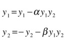
To do this, we create the function lotka in the M-file lotka.m as depicted in Figure 7-14.

Later, we might type the following in the command line:
>> global ALPHA BETA
ALPHA = 0.01
BETA = 0.02
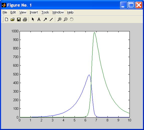
These global values may then be used for α and β in the M-file lotka.m (without having to specify them). For example, we can generate the graph (Figure 7-15) with the following syntax:
>> [t, y] = ode23 ('lotka', 0.10, [1; 1]); plot(t,y)
7.6 Data Types
MATLAB has 14 different data types, summarized in Figure 7-16 below.

Below are the different types of data:
Data type | Example | Description |
|---|---|---|
single |
3* 10 ^ 38 |
Simple numerical precision. This requires less storage than double precision, but it is less precise. This type of data should not be used in mathematical operations. |
Double |
3*10^300 5+6i |
Double numerical precision. This is the most commonly used data type in MATLAB. |
sparse |
speye(5) |
Sparse matrix with double precision. |
int8, uint8, int16, uint16, int32, uint32 |
UInt8(magic (3)) |
Integers and unsigned integers with 8, 16, and 32 bits. These make it possible to use entire amounts with efficient memory management. This type of data should not be used in mathematical operations. |
char |
'Hello' |
Characters (each character has a length of 16 bits). |
cell |
{17 'hello' eye (2)} |
Cell (contains data of similar size) |
structure |
a.day = 12; a.color = 'Red'; a.mat = magic(3); |
Structure (contains cells of similar size) |
user class |
inline('sin (x)') |
MATLAB class (built with functions) |
java class |
Java. awt.Frame |
Java class (defined in API or own) with Java |
function handle |
@humps |
Manages functions in MATLAB. It can be last in a list of arguments and evaluated with feval. |
7.7 Flow Control: FOR, WHILE and IF ELSEIF Loops
The use of recursive functions, conditional operations and piecewise defined functions is very common in mathematics. The handling of loops is necessary for the definition of these types of functions. Naturally, the definition of the functions will be made via M-files.
7.8 FOR Loops
MATLAB has its own version of the DO statement (defined in the syntax of most programming languages). This statement allows you to run a command or group of commands repeatedly. For example:
>> for i=1:3, x(i)=0, end
x =
0
x =
0     0
x =
0 0 0
The general form of a FOR loop is as follows:
for variable = expression
commands
end
The loop always starts with the clause for and ends with the clause end, and includes in its interior a whole set of commands that are separated by commas. If any command defines a variable, it must end with a semicolon in order to avoid repetition in the output. Typically, loops are used in the syntax of M-files. Here is an example (Figure 7-17):

In this loop we have defined a Hilbert matrix of order (m, n). If we save it as an M-file matriz.m, we can build any Hilbert matrix later by running the M-file and specifying values for the variables m and n (the matrix dimensions) as shown below:
>> M = matriz (4,5)

M =

1.0000 0.5000 0.3333 0.2500 0.2000
0.5000 0.3333 0.2500 0.2000 0.1667
0.3333 0.2500 0.2000 0.1667 0.1429
0.2500 0.2000 0.1667 0.1429 0.1250
7.9 WHILE Loops
MATLAB has its own version of the WHILE structure defined in the syntax of most programming languages. This statement allows you to repeat a command or group of commands a number of times while a specified logical condition is met. The general syntax of this loop is as follows:
While condition
commands
end
The loop always starts with the clause while, followed by a condition, and ends with the clause end, and includes in its interior a whole set of commands that are separated by commas which continually loop while the condition is met. If any command defines a variable, it must end with a semicolon in order to avoid repetition in the output. As an example, we write an M-file (Figure 7-18) that is saved as while1.m, which calculates the largest number whose factorial does not exceed 10100.

Now now run the M-file.
>> while1

n =

    70
7.10 IF ELSEIF ELSE END Loops
MATLAB, like most structured programming languages, also includes the IF-ELSEIF-ELSE-END structure. Using this structure, scripts can be run if certain conditions are met. The loop syntax is as follows:
if condition
commands
end
In this case the commands are executed if the condition is true. But the syntax of this loop may be more general.
if condition
    commands1
else
    commands2
end
In this case, the commands commands1 are executed if the condition is true, and the commands commands2 are executed if the condition is false.
IF statements and FOR statements can be nested. When multiple IF statements are nested using the ELSEIF statement, the general syntax is as follows:
if condition1
    commands1
elseif condition2
    commands2
elseif condition3
    commands3
.
.
else
end
In this case, the commands commands1 are executed if condition1 is true, the commands commands2 are executed if condition1 is false and condition2 is true, the commands commands3 are executed if condition1 and condition2 are false and condition3 is true, and so on.
The previous nested syntax is equivalent to the following unnested syntax, but executes much faster:
if condition1
    commands1
else
      if condition2
          commands2
      else
            if condition3
                commands3
            else
            .
            .
            .
            end
       end
end
Consider, for example, the M-file else1.m (see Figure 7-19).
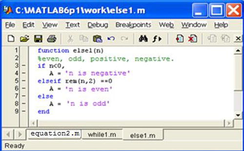
When you run the file it returns negative, odd or even according to whether the argument n is negative, non-negative and odd, or non-negative and even, respectively:
>> else1 (8), else1 (5), else1 (-10)

A =

n is even

A =

n is odd

A =

n is negative
7.11 SWITCH and CASE
The switch statement executes certain statements based on the value of a variable or expression. Its basic syntax is as follows:
switch expression (scalar or string)
case value1
statements % runs if expression is value1
case value2
statements % runs if expression is value2
.
.
.
otherwise
statements % runs if neither case is satisfied

end
Below is an example of a function that returns ‘minus one’, ‘zero’, ‘one’, or ‘another value’ according to whether the input is equal to -1,0,1 or something else, respectively (Figure 7-20).

Running the above example we get:
>> case1 (25)
another value

>> case1 (- 1)
minus one
7.12 CONTINUE
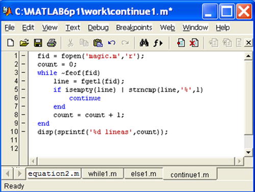
The continue statement passes control to the next iteration in a for loop or while loop in which it appears, ignoring the remaining instructions in the body of the loop. Below is an M-file continue.m (Figure 7-21) that counts the lines of code in the file magic.m, ignoring the white lines and comments.

Running the M-file, we get:
>> continue1
25 lines
7.13 BREAK
The break statement terminates the execution of a for loop or while loop, skipping to the first instruction which appears outside of the loop. Below is an M-file break1.m (Figure 7-22) which reads the lines of code in the file fft.m, exiting the loop as soon as it encounters the first empty line.
Running the M-file we get:
>> break1

%FFT Discrete Fourier transform.
%   FFT(X) is the discrete Fourier transform (DFT) of vector X.  For
%   matrices, the FFT operation is applied to each column. For N-D
%   arrays, the FFT operation operates on the first non-singleton
%   dimension.
%
%   FFT(X,N) is the N-point FFT, padded with zeros if X has less
%   than N points and truncated if it has more.
%
%   FFT(X,[],DIM) or FFT(X,N,DIM) applies the FFT operation across the
%   dimension DIM.
%
%   For length N input vector x, the DFT is a length N vector X,
%   with elements
%                    N
%      X(k) =       sum  x(n)*exp(-j*2*pi*(k-1)*(n-1)/N), 1 <= k <= N.
%                   n=1
%   The inverse DFT (computed by IFFT) is given by
%                    N
%      x(n) = (1/N) sum  X(k)*exp( j*2*pi*(k-1)*(n-1)/N), 1 <= n <= N.
%                   k=1
%
%   See also IFFT, FFT2, IFFT2, FFTSHIFT.
7.14 TRY ... CATCH
The instructions between try and catch are executed until an error occurs. The instruction lasterr is used to show the cause of the error. The general syntax of the command is as follows:
try,
instruction
...,
instruction
catch,
instruction
...,
instruction
end
7.15 RETURN
The return statement terminates the current script and returns the control to the invoked function or the keyboard. The following is an example (Figure 7-23) that computes the determinant of a non-empty matrix. If the array is empty it returns the value 1.
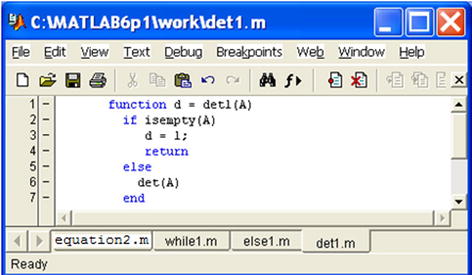
Running the function for a non-empty array we get:
>> A = [- 1, - 1, 1; 1,0,1; 1,1,1]


A =
-1 -1 -1
 1  0  1
 1 -1 -1

>> det1 (A)

ans =

2
Now we apply the function to an empty array:
>> B =[]

B =

     []

>> det1 (B)

ans =

     1
7.16 Subfunctions
M-file-defined functions can contain code for more than one function. The main function in an M-file is called a primary function, which is precisely the function which invokes the M-file, but subfunctions hanging from the primary function may be added which are only visible for the primary function or another subfunction within the same M-file. Each subfunction begins with its own function definition. An example is shown in Figure 7-24.

The subfunctions mean and median calculate the arithmetic mean and the median of the input list. The primary function newstats determines the length n of the list and calls the subfunctions with the list as the first argument and n as the second argument. When executing the main function, it is enough to provide as input a list of values for which the arithmetic mean and median will be calculated. The subfunctions are executed automatically, as shown below.
>> [mean, median] = newstats ([10,20,3,4,5,6])

mean =

     8

median =

    5.5000
7.17 Commands in M-files
MATLAB provides certain procedural commands which are often used in M-file scripts. Among them are the following:
echo on |
View on-screen commands of an M-file script while it is running. |
echo off |
Hides on-screen commands of an M-file script (this is the default setting). |
pause |
Interrupts the execution of an M-file until the user presses a key to continue. |
pause(n) |
Interrupts the execution of an M-file for n seconds. |
pause off |
Disables pause and pause (n). |
pause on |
Enables pause and pause (n). |
keyboard |
Interrupts the execution of an M-file and passes the control to the keyboard so that the user can perform other tasks. The execution of the M-file can be resumed by typing the return command into the Command Window and pressing Enter. |
return |
Resumes execution of an M-file after an outage. |
break |
Prematurely exits a loop. |
CLC |
Clears the Command Window. |
Home |
Hides the cursor. |
more on |
Enables paging of the MATLAB Command Window output. |
more off |
Disables paging of the MATLAB Command Window output. |
more(N) |
Sets page size to N lines. |
menu |
Offers a choice between various types of menu for user input. |
7.18 Functions relating to Arrays of Cells
An array is a well-ordered collection of individual items. It is simply a list of elements, each of which is associated with a positive integer called its index, which represents the position of that element in the list. It is essential that each element is associated with a unique index, which can be zero or negative, which identifies it fully, so that to make changes to any elements of the array it suffices to refer to their indices. Arrays can be of one or more dimensions, and correspondingly they have one or more sets of indices that identify their elements. The most important commands and functions that enable MATLAB to work with arrays of cells are the following:
c = cell(n) c = cell(m,n) c = cell([m n]) c = cell(m,n,p,...) c = cell([m n p ...]) c = cell(size(A)) |
Creates an n×n array whose cells are empty arrays. Creates an m×n array whose cells are empty arrays. Creates an m×n array whose cells are empty arrays. Creates an m×n×p×... array of empty arrays. Creates an m×n×p×... array of empty arrays. Creates an array of empty arrays of the same size as A. |
D = cellfun('f',C) D = cellfun('size',C,k) D = cellfun('isclass',C,class) |
Applies the function f (isempty, islogical, isreal, length, ndims, or prodofsize) to each element of the array C. Returns the size of each element of dimension k in C. Returns true for each element of C corresponding to class. |
C=cellstr(S) |
Places each row of the character array S into separate cells of C. |
S = cell2struct(C,fields,dim) |
Converts the array C to a structure array S incorporating field names ‘fields’ and the dimension ‘dim’ of C. |
celldisp (C) celldisp(C, name) |
Displays the contents of the array C. Assigns the contents of the array C to the variable name. |
cellplot(C) cellplot(C,'legend') |
Shows a graphical representation of the array C. Shows a graphical representation of the array C and incorporates a legend. |
C = num2cell(A) C = num2cell(A,dims) |
Converts a numeric array A to the cell array C Converts a numeric array A to a cell array C placing the given dimensions in separate cells. |
As a first example, we create an array of cells of the same size as the unit square matrix of order two.
>> A = ones(2,2)

A =
1     1
1     1

>> c = cell(size(A))

c =

[]     []
[]     []
We then define and present a 2 × 3 array of cells element by element, and apply various functions to the cells.
>> C{1.1} = [1 2; 4 5];
C{1,2} = 'Name';
C{1,3} = pi;
C{2,1} = 2 + 4i;
C{2,2} = 7;
C{2,3} = magic(3);

>> C

C =

[2x2 double]    'Name'    [    3.1416]
[2.0000+ 4.0000i]    [   7]    [3x3 double]

>> D = cellfun('isreal',C)

D =

1     1     1
0     1     1

>> len = cellfun('length',C)

len =

2     4     1
1     1     3

>> isdbl = cellfun('isclass',C,'double')

isdbl =

1 0 1
1 1 1
The contents of the cells in the array C defined above are revealed using the command celldisp.
>> celldisp(C)

C{1,1} =
1     2
4     5

C{2,1} =

2.0000 + 4.0000i

C{1,2} =

Name

C {2,2} =

7

C {1,3} =

3.1416


C {2,3} =

8 1 6
3 5 7
4 9 2
The following displays a graphical representation of the array C (Figure 7-25).
>> cellplot(C)

7.19 Functions of Multidimensional Arrays
The following group of functions is used by MATLAB to work with multidimensional arrays:
C = cat(dim,A,B) C = cat(dim,A1,A2,A3,A4...) |
Concatenates arrays A and B according to the dimension dim. Concatenates arrays A1, A2,... according to the dimension dim. |
B = flipdim (A, dim) |
Flips the array A along the specified dimension dim. |
[I,J] = ind2sub(siz,IND) [I1,I2,I3,...,In] = ind2sub(siz,IND) |
Returns the matrices I and J containing the equivalent row and column subscripts corresponding to each index in the matrix IND for a matrix of size siz. Returns matrices I1, I2,...,In containing the equivalent row and column subscripts corresponding to each index in the matrix IND for a matrix of size siz. |
A = ipermute(B,order) |
Inverts the dimensions of the multidimensional array D according to the values of the vector order. |
[X1, X2, X3,...] = ndgrid(x1,x2,x3,...) [X 1, X 2,...] = ndgrid (x) |
Transforms the domain specified by vectors x1, x2,... into the arrays X1, X2,... which can be used for evaluation of functions of several variables and interpolation. Equivalent to ndgrid(x,x,x,...). |
n = ndims(A) |
Returns the number of dimensions in the array A. |
B = permute(A,order) |
Swaps the dimensions of the array A specified by the vector order. |
B = reshape(A,m,n) B = reshape(A,m,n,p,...) B = reshape(A,[m n p...]) B = reshape(A,siz) |
Defines an m×n matrix B whose elements are the columns of a. Defines an array B whose elements are those of the array A restructured according to the dimensions m×n×p×... Equivalent to B = reshape(A,m,n,p,...) Defines an array B whose elements are those of the array A restructured according to the dimensions of the vector siz. |
B = shiftdim(X,n) [B,nshifts] = shiftdim(X) |
Shifts the dimensions of the array X by n, creating a new array B. Defines an array B with the same number of elements as X but with leading singleton dimensions removed. |
B=squeeze(A) |
Creates an array B with the same number of elements as A but with all singleton dimensions removed. |
IND = sub2ind(siz,I,J) IND = sub2ind(siz,I1,I2,...,In) |
Gives the linear index equivalent to the row and column indices I and J for a matrix of size siz. Gives the linear index equivalent to the n indices I1, I2,..., in a matrix of size siz. |
As a first example we concatenate a magic square and Pascal matrix of order 3.
>> A = magic (3); B = pascal (3);
>> C = cat (4, A, B)

C(:,:,1,1) =

8 1 6
3 5 7
4 9 2


C(:,:,1,2) =

1 1 1
1 2 3
1 3 6
The following example flips the Rosser matrix.
>> R=rosser

R =

   611   196  -192   407    -8   -52   -49    29
   196   899   113  -192   -71   -43    -8   -44
  -192   113   899   196    61    49     8    52
   407  -192   196   611     8    44    59   -23
    -8   -71    61     8   411  -599   208   208
   -52   -43    49    44  -599   411   208   208
   -49    -8     8    59   208   208    99  -911
    29   -44    52   -23   208   208  -911    99

>> flipdim(R,1)

ans =

ans =

    29   -44    52   -23   208   208  -911    99
   -49    -8     8    59   208   208    99  -911
   -52   -43    49    44  -599   411   208   208
    -8   -71    61     8   411  -599   208   208
   407  -192   196   611     8    44    59   -23
  -192   113   899   196    61    49     8    52
   196   899   113  -192   -71   -43    -8   -44
   611   196  -192   407    -8   -52   -49    29
Now we define an array by concatenation and permute and inverse permute its elements.
>> a = cat(3,eye(2),2*eye(2),3*eye(2))


a(:,:,1) =

1 0
0 1


a(:,:,2) =

2 0
0 2


a(:,:,3) =

3 0
0 3

>> B = permute(a,[3 2 1])

B(:,:,1) =

1 0
2 0
3 0

B(:,:,2) =

0 1
0 2
0 3

>> C = ipermute(B,[3 2 1])

C(:,:,1) =

1 0
0 1

C(:,:,2) =

2 0
0 2

C(:,:,3) =

3 0
0 3
The following example evaluates the function ![]() in the square [-2, 2] × [-2, 2] and displays it graphically (Figure 7-26).
in the square [-2, 2] × [-2, 2] and displays it graphically (Figure 7-26).
>> [X 1, X 2] = ndgrid(-2:.2:2,-2:.2:2);
Z = X 1. * exp(-X1.^2-X2.^2);
mesh (Z)

In the following example we resize a 3 × 4 random matrix to a 2 × 6 matrix.
>> A = rand(3,4)

A =

0.9501    0.4860    0.4565    0.4447
0.2311    0.8913    0.0185    0.6154
0.6068    0.7621    0.8214    0.7919

>> B = reshape(A,2,6)

B =

   0.9501 0.6068 0.8913 0.4565 0.8214 0.6154
   0.2311 0.4860 0.7621 0.0185 0.4447 0.7919
7.20 Numerical Analysis Methods in MATLAB
MATLAB programming techniques allow you to implement a wide range of numerical algorithms. It is possible to design programs which perform numerical integration and differentiation, solve differential equations, optimize non-linear functions, etc. However, MATLAB’s Basic module already has a number of tailor-made functions which implement some of these algorithms. These functions are set out in the following subsections. In the next chapter we will give some examples showing how these functions can be used in practice.
7.21 Zeros of Functions and Optimization
The commands (functions) that enables MATLAB’s Basic module to optimize functions and find the zeros of functions are as follows:
x = fminbnd(fun,x1,x2) |
Minimizes the function on the interval (x1 x2). |
x = fminbnd(fun,x1,x2,options) |
Minimizes the function on the interval (x1 x2) according to the option given by optimset (...). This last command is explained later. |
x = fminbnd(fun,x1,x2,options,P1,P2,...) |
Specifies additional parameters P1, P2,... to pass to the target function fun(x,P1,P2,...). |
[x, fval] = fminbnd (...) |
Returns the value of the objective function at x. |
[x, fval, f] = fminbnd (...) |
In addition, returns an indicator of convergence f (f > 0 indicates convergence to the solution, f < 0 indicates no convergence and f = 0 indicates the algorithm exceeded the maximum number of iterations). |
[x,fval,f,output] = fminbnd(...) |
Provides further information (output.algorithm gives the algorithm used, output.funcCount gives the number of evaluations of fun and output.iterations gives the number of iterations). |
x = fminsearch(fun,x0) x = fminsearch(fun,x0,options) x = fminsearch(fun,x0,options,P1,P2,...) [x,fval] = fminsearch(...) [x,fval,f] = fminsearch(...) [x,fval,f,output] = fminsearch(...) |
Returns the minimum of a scalar function of several variables, starting at an initial estimate x0. The argument x0 can be an interval [a, b]. To find the minimum of fun in [a, b], x = fminsearch (fun, [a, b]) is used. |
x = fzero(fun,x0) x = fzero(fun,x0,options) x = fzero(fun,x0,options,P1,P2,...) [x, fval] = fzero (...) [x, fval, exitflag] = fzero (...) [x,fval,exitflag,output] = fzero(...) |
Finds zeros of the function fun, with initial estimate x0, by finding a point where fun changes sign. The argument x0 can be an interval [a, b]. Then, to find a zero of fun in [a, b], we use x = fzero (fun, [a, b]), where fun has opposite signs at a and b. |
options = optimset('p1',v1,'p2',v2,...) |
Creates optimization parameters p1, p2,... with values v1, v2... The possible parameters are Display (with possible values 'off', 'iter','final','notify') to respectively not display the output, display the output of each iteration, display only the final output, and display a message if there is no convergence); MaxFunEvals, whose value is an integer indicating the maximum number of evaluations; MaxIter whose value is an integer indicating the maximum number of iterations; TolFun, whose value is an integer indicating the tolerance in the value of the function, and TolX, whose value is an integer indicating the tolerance in the value of x. |
val = optimget (options, 'param') |
Returns the value of the parameter specified in the optimization options structure. |
g = inline (expr) |
Transforms the string expr into a function. |
g = inline(expr,arg1,arg2, ...) |
Transforms the string expr into a function with given input arguments. |
g = inline (expr, n) |
Transforms the string expr into a function with n input arguments. |
f = @function |
Enables the function to be evaluated. |
As a first example we find the value of x that minimizes the function cos(x) in the interval (3,4).
>> x = fminbnd(@cos,3,4)

x =
3.1416
We could also have used the following syntax:
>> x = fminbnd(inline('cos(x)'),3,4)

x =
3.1416
In the following example we find the above minimum to 8 decimal places and find the value of x that minimizes the cosine in the given interval, presenting information relating to all iterations of the process.
>> [x,fval,f] = fminbnd(@cos,3,4,optimset('TolX',1e-8,...          'Display','iter'));


Func-count     x          f(x)       Procedure
1        3.38197    -0.971249        initial
2        3.61803    -0.888633        golden
3        3.23607    -0.995541        golden
4        3.13571    -0.999983        parabolic
5         3.1413           -1        parabolic
6        3.14159           -1        parabolic
7        3.14159           -1        parabolic
8        3.14159           -1        parabolic
9        3.14159           -1        parabolic

Optimization terminated successfully:
the current x satisfies the termination criteria using OPTIONS.TolX of 1.000000e-008
In the following example, taking (- 1, 2; 1) as initial values, we find the minimum and target value of the following function of two variables:
![]()
>> [x,fval] = fminsearch(inline('100*(x(2)-x(1)^2)^2+...
(((1-x (1)) ^ 2'), [- 1.2, 1])

x =

1.0000 1.0000


fval =

8. 1777e-010
The following example computes a zero of the sine function with an initial estimate of 3, and a zero of the cosine function between 1 and 2.
>> x = fzero(@sin,3)

x =

3.1416

>> x = fzero(@cos,[1 2])

x =

    1.5708
7.22 Numerical Integration
MATLAB contains functions that allow you to perform numerical integration using Simpson’s method and Lobatto’s method. The syntax of these functions is as follows:
q = quad(f,a,b) |
Finds the integral of f between a and b by Simpson’s method with an error of 10-6. |
q = quad(f,a,b,tol) |
Find the integral of f between a and b by Simpson’s method with the tolerance tol instead of 10-6. |
q = quad(f,a,b,tol,trace) |
Find the integral of f between a and b by Simpson’s method with the tolerance tol and presents the trace of iterations. |
q = quad(f,a,b,tol,trace,p1,p2,...) |
Passes additional arguments p1, p2,... to the function f, f(x,p1,p2,...). |
[q, fcnt] = quadl(f,a,b,...) |
Additionally returns the number of evaluations of f. |
q = quadl(f,a,b) |
Finds the integral of f between a and b by Lobatto’s quadrature method with a 10-6 error. |
q = quadl(f,a,b,tol) |
Finds the integral of f between a and b by Lobatto’s quadrature method with the tolerance tol instead of 10-6. |
q = quadl(f,a,b,tol,trace) |
Finds the integral of f between a and b by Lobatto’s quadrature method with the tolerance tol and presents the trace of iterations. |
q = quad(f,a,b,tol,trace,p1,p2,...) |
Passes additional arguments p1, p2,... to the function f, f(x,p1,p2,...). |
[q, fcnt] = quadl(f,a,b,...) |
Additionally returns the number of evaluations of f. |
q = dblquad (f, xmin, xmax, ymin, ymax) |
Evaluates the double integral f(x,y) in the rectangle specified by the given parameters, with an error of 10-6. dblquad will be removed in future releases and replaced by integral2. |
q = dblquad (f, xmin, xmax, ymin,ymax,tol) |
Evaluates the double integral f(x,y) in the rectangle specified by the given parameters, with tolerance tol. |
q = dblquad (f, xmin, xmax, ymin,ymax,tol,@quadl) |
Evaluates the double integral f(x,y) in the rectangle specified by the given parameters, with tolerance tol and using the quadl method. |
q = dblquad (f, xmin, xmax, ymin,ymax,tol,method,p1,p2,...) |
Passes additional arguments p1, p2,... to the function f. |
As a first example, we calculate  using Simpson’s method.
>> F = inline('1./(x.^3-2*x-5)');
>> Q = quad(F,0,2)

Q =

-0.4605
Then we observe that the integral remains unchanged even if we increase the tolerance to 10-18.
>> Q = quad(F,0,2,1.0e-18)

Q =

-0.4605
In the following example we evaluate the same integral using Lobatto’s method.
>> Q = quadl(F,0,2)

Q =

-0.4605
We evaluate the double integral  .
.
>> Q = dblquad (inline (' y * sin (x) + x * cos (y)'), pi, 2 * pi, 0, pi)

Q =

   -9.8696
7.23 Numerical Differentiation
The derivative f'(x) of a function f (x) can simply be defined as the rate of change of f (x) with respect to x. The derivative can be expressed as a ratio between the change in f (x), denoted by df (x), and the change in x, denoted by dx. The derivative of a function f at the point xk can be estimated by using the expression:

provided the values xk, xk-1 are close to each other. Similarly the second derivative f''(x) of the function f(x) can be estimated as the first derivative of f'(x), i.e.:

MATLAB includes in its Basic module the function diff, which allows you to approximate derivatives. The syntax is as follows:
Y = diff(X) |
Calculates the differences between adjacent elements in the vector X:[X(2) - X(1), X(3) - X (2),..., X(n) - X(n-1)]. If X is an m×n matrix, diff (X) returns the array of differences by rows: [X(2:m,:)-X(1:m-1,:)] |
Y = diff(X,n) |
Finds differences of order n, for example: diff(X,2) = diff (diff (X)). |
As an example we consider the function f(x) = x5-3x4-11x3+27x2+10x-24, find the difference vector of [-4,-3.9,-3.8,...,4.8,4.9,5] the difference vector of [f(-4),f(-3.9),f(-3.8),...,f(4.8),f(4.9),f(5)] and the elementwise quotient of the latter by the former, and graph the function in the interval [-4,5]. See Figure 7-27.
>> x =-4:0.1: 5;
>> f = x.^5-3*x.^4-11*x.^3 + 27*x.^2 + 10*x-24;
>> df=diff(f)./diff(x)

df =

  1.0e+003 *

  Columns 1 through 7

    1.2390    1.0967    0.9655    0.8446    0.7338    0.6324    0.5400

  Columns 8 through 14

    0.4560    0.3801    0.3118    0.2505    0.1960    0.1477    0.1053

  Columns 15 through 21

    0.0683    0.0364    0.0093   -0.0136   -0.0324   -0.0476   -0.0594

  Columns 22 through 28

   -0.0682   -0.0743   -0.0779   -0.0794   -0.0789   -0.0769   -0.0734

  Columns 29 through 35

   -0.0687   -0.0631   -0.0567   -0.0497   -0.0424   -0.0349   -0.0272

  Columns 36 through 42

   -0.0197   -0.0124   -0.0054    0.0012    0.0072    0.0126    0.0173

  Columns 43 through 49

    0.0212    0.0244    0.0267    0.0281    0.0287    0.0284    0.0273

  Columns 50 through 56

    0.0253    0.0225    0.0189    0.0147    0.0098    0.0044   -0.0014

  Columns 57 through 63

   -0.0076   -0.0140   -0.0205   -0.0269   -0.0330   -0.0388   -0.0441

  Columns 64 through 70

   -0.0485   -0.0521   -0.0544   -0.0553   -0.0546   -0.0520   -0.0472

  Columns 71 through 77

-0.0400   -0.0300   -0.0170   -0.0007    0.0193    0.0432    0.0716

  Columns 78 through 84

    0.1046    0.1427    0.1863    0.2357    0.2914    0.3538    0.4233

  Columns 85 through 90

    0.5004    0.5855    0.67910.7816    0.8936    1.0156

>> plot (x, f)

7.24 Approximate Solutions of Differential Equations
MATLAB provides commands in its Basic module allowing for the numerical solution of ordinary differential equations (ODEs), differential algebraic equations (DAEs) and boundary value problems. It is also possible to solve systems of differential equations with boundary values and parabolic and elliptic partial differential equations.
7.25 Ordinary Differential Equations with Initial Values
An ordinary differential equation contains one or more derivatives of the dependent variable y with respect to the independent variable t. A first order ordinary differential equation with an initial value for the independent variable can be represented as:

The previous problem can be generalized to the case where y is a vector, y = (y1, y2,...,yn).
MATLAB’s Basic module commands relating to ordinary differential equations and differential algebraic equations with initial values are presented in the following table:
Command |
Class of problem solving, numerical method and syntax |
|---|---|
ode45 |
Ordinary differential equations by the Runge–Kutta method |
ode23 |
Ordinary differential equations by the Runge–Kutta method |
ode113 |
Ordinary differential equations by Adams’ method |
ode15s |
Differential algebraic equations and ordinary differential equations using NDFs (BDFs) |
ode23s |
Ordinary differential equations by the Rosenbrock method |
ode23t |
Ordinary differential and differential algebraic equations by the trapezoidal rule |
ode23tb |
Ordinary differential equations using TR-BDF2 |
The common syntax for the previous seven commands is the following:
[T, y] = solver(odefun,tspan,y0)
[T, y] = solver(odefun,tspan,y0,options)
[T, y] = solver(odefun,tspan,y0,options,p1,p2...)
[T, y, TE, YE, IE] = solver(odefun,tspan,y0,options)
In the above, solver can be any of the commands ode45, ode23, ode113, ode15s, ode23s, ode23t, or ode23tb.
The argument odefun evaluates the right-hand side of the differential equation or system written in the form y' = f (t, y) or M(t, y)y '=f (t, y), where M(t, y) is called a mass matrix. The command ode23s can only solve equations with constant mass matrix. The commands ode15s and ode23t can solve algebraic differential equations and systems of ordinary differential equations with a singular mass matrix. The argument tspan is a vector that specifies the range of integration [t0, tf] (tspan= [t0, t1,...,tf], which must be either an increasing or decreasing list, is used to obtain solutions for specific values of t). The argument y0 specifies a vector of initial conditions. The arguments p1, p2,... are optional parameters that are passed to odefun. The argument options specifies additional integration options using the command options odeset which can be found in the program manual. The vectors T and Y present the numerical values of the independent and dependent variables for the solutions found.
As a first example we find solutions in the interval [0,12] of the following system of ordinary differential equations:

For this, we define a function named system1 in an M-file, which will store the equations of the system. The function begins by defining a column vector with three rows which are subsequently assigned components that make up the syntax of the three equations (Figure 7-28).

We then solve the system by typing the following in the Command Window:
>> [T, Y] = ode45(@system1,[0 12],[0 1 1])

T =

0
0.0001
0.0001
0.0002
0.0002
0.0005
.
.
11.6136
11.7424
11.8712
12.0000

Y =
0 1.0000 1.0000
0.0001 1.0000 1.0000
0.0001 1.0000 1.0000
0.0002 1.0000 1.0000
0.0002 1.0000 1.0000
0.0005 1.0000 1.0000
0.0007 1.0000 1.0000
0.0010 1.0000 1.0000
0.0012 1.0000 1.0000
0.0025 1.0000 1.0000
0.0037 1.0000 1.0000
0.0050 1.0000 1.0000
0.0062 1.0000 1.0000
0.0125 0.9999 1.0000
0.0188 0.9998 0.9999
0.0251 0.9997 0.9998
0.0313 0.9995 0.9997
0.0627 0.9980 0.9990
.
.
0.8594  -0.5105 0.7894
0.7257  -0.6876 0.8552
0.5228  -0.8524 0.9281
0.2695  -0.9631 0.9815
-0.0118 -0.9990 0.9992
-0.2936 -0.9540 0.9763
-0.4098 -0.9102 0.9548
-0.5169 -0.8539 0.9279
-0.6135 -0.7874 0.8974
-0.6987 -0.7128 0.8650
To better interpret the results, the above numerical solution can be graphed (Figure 7-29) by using the following command:
>> plot (T, Y(:,1), '-', T, Y(:,2),'-', T, Y(:,3),'. ')

7.26 Ordinary Differential Equations with Boundary Conditions
MATLAB also allows you to solve ordinary differential equations with boundary conditions. The boundary conditions specify a relationship that must hold between the values of the solution function at the end points of the interval on which it is defined. The simplest problem of this type is the system of equations
![]()
where x is the independent variable, y is the dependent variable and y' is the derivative with respect to x (i.e., y'= dy/dx). In addition, the solution on the interval [a, b] has to meet the following boundary condition:
![]()
More generally this type of differential equation can be expressed as follows:

where the vector p consists of parameters which have to be determined simultaneously with the solution via the boundary conditions.
The command that solves these problems is bvp4c, whose syntax is as follows:
Sol = bvp4c (odefun, bcfun, solinit)
Sol = bvp4c (odefun, bcfun, solinit, options)
Sol = bvp4c(odefun,bcfun,solinit,options,p1,p2...)
In the syntax above odefun is a function that evaluates f (x, y). It may take one of the following forms:
dydx = odefun(x,y)
dydx = odefun(x,y,p1,p2,...)
dydx = odefun (x, y, parameters)
dydx = odefun(x,y,parameters,p1,p2,...)
The argument bcfun in Bvp4c is a function that computes the residual in the boundary conditions. Its form is as follows:
Res = bcfun (ya, yb)
Res = bcfun(ya,yb,p1,p2,...)
Res = bcfun (ya, yb, parameters)
Res = bcfun(ya,yb,parameters,p1,p2,...)
The argument solinit is a structure containing an initial guess of the solution. It has the following fields: x (which gives the ordered nodes of the initial mesh so that the boundary conditions are imposed at a = solinit.x(1)and b = solinit.x(end)) and y (the initial guess for the solution, given as a vector, so that the i-th entry is a constant guess for the i-th component of the solution at all the mesh points given by x). The structure solinit is created using the command bvpinit. The syntax is solinit = bvpinit(x,y).
As an example we solve the second order differential equation:
![]()
whose solutions must satisfy the boundary conditions:

This is equivalent to the following problem (where y1=y and y2=y'):

We consider a mesh of five equally spaced points in the interval [0,4] and our initial guess for the solution is y1 = 1 and y2 = 0. These assumptions are included in the following syntax:
>> solinit = bvpinit (linspace (0,4,5), [1 0]);
The M-files depicted in Figures 7-30 and 7-31 show how to enter the equation and its boundary conditions.


The following syntax is used to find the solution of the equation:
>> Sun = bvp4c (@twoode, @twobc, solinit);
The solution can be graphed (Figure 7-32) using the command bvpval as follows:
>> y = bvpval (Sun, linspace (0,4));
>> plot (x, y(1,:));

7.27 Partial Differential Equations
MATLAB’s Basic module has features that enable you to solve partial differential equations and systems of partial differential equations with initial boundary conditions. The basic function used to calculate the solutions is pedepe, and the basic function used to evaluate these solutions is pdeval.
The syntax of the function pedepe is as follows:
Sol = pdepe (m, pdefun, icfun, bcfun, xmesh, tspan)
Sol = pdepe (m, pdefun, icfun, bcfun, xmesh, tspan, options)
Sun = pdepe(m,pdefun,icfun,bcfun,xmesh,tspan,options,p1,p2...)
The parameter m takes the value 0, 1 or 2 according to the nature of the symmetry of the problem (block, cylindrical or spherical, respectively). The argument pdefun defines the components of the differential equation, icfun defines the initial conditions, bcfun defines the boundary conditions, xmesh and tspan are vectors [x0, x1,...,xn] and [t0, t1,...,tf] that specify the points at which a numerical solution is requested (n, f≥3), options specifies some calculation options of the underlying solver (RelTol, AbsTol,NormControl, InitialStep and MaxStep to specify relative tolerance, absolute tolerance, norm tolerance, initial step and max step, respectively) and p1, p2,... are parameters to pass to the functions pdefun, icfun and bcfun.
pdepe solves partial differential equations of the form:

where a≤x≤b and t0≤t≤tf. Moreover, for t = t0 and for all x the solution components meet the initial conditions:
![]()
and for all t and each x = a or x = b, the solution components satisfy the boundary conditions of the form:

In addition, we have that a = xmesh (1), b = xmesh (end), tspan (1) =t0 and tspan (end) = tf. Moreover pdefun finds the terms c, f and s of the partial differential equation, so that:
[c, f, s] = pdefun (x, t, u, dudx)
Similiarly icfun evaluates the initial conditions
u = icfun (x)
Finally, bcfun evaluates the terms p and q of the boundary conditions:
[pl, ql, pr, qr] = bcfun (xl, ul, xr, ur, t)
As a first example we solve the following partial differential equation (x![]() [0,1] and t≥0):
[0,1] and t≥0):

satisfying the initial condition:
![]()
and the boundary conditions:

We begin by defining functions in M-files as shown in Figures 7-33 to 7-35.


Once the support functions have been defined, we define the function that solves the equation (see the M-file in Figure 7-36).

To view the solution (Figures 7-37 and 7-38), we enter the following into the MATLAB Command Window:
>> pdex1


As a second example we solve the following system of partial differential equations (x![]() [0,1] and t≥0):
[0,1] and t≥0):

![]()
satisfying the initial conditions:

and the boundary conditions:

To conveniently use the function pdepe, the system can be written as:

The left boundary condition can be written as:

and the right boundary condition can be written as:

We start by defining the functions in M-files as shown in Figures 7-39 to 7-41.


Once the support functions are defined, the function that solves the system of equations is given by the M-file shown in Figure 7-42.

To view the solution (Figures 7-43 and 7-44), we enter the following in the MATLAB Command Window:
>> pdex4


EXERCISE 7-1
Minimize the function x3-2x-5 in the interval (0,2) and calculate the value that the function takes at that point, displaying information about all iterations of the optimization process.
>> f = inline('x.^3-2*x-5');
>> [x,fval] = fminbnd(f, 0, 2,optimset('Display','iter'))
Func-count x f(x) Procedure
1 0.763932 -6.08204 initial
2 1.23607 -5.58359 golden
3 0.472136 -5.83903 golden
4 0.786475 -6.08648 parabolic
5 0.823917 -6.08853 parabolic
6 0.8167 -6.08866 parabolic
7 0.81645 -6.08866 parabolic
8 0.816497 -6.08866 parabolic
9 0.81653 -6.08866 parabolic
Optimization terminated successfully:
the current x satisfies the termination criteria using OPTIONS.TolX of 1.000000e-004
x =
0.8165
fval =
-6.0887
EXERCISE 7-2
Find in a neighborhood of x = 1.3 a zero of the function:

Minimize this function on the interval (0,2).
First we find a zero of the function using the initial estimate of x= 1.3, presenting information about the iterations and checking that the result is indeed a zero.
>> [x,feval]=fzero(inline('1/((x-0.3)^2+0.01)+...
1/((x-0.9)^2+0.04)-6'),1.3,optimset('Display','iter'))
Func-count x f(x) Procedure
1 1.3 -0.00990099 initial
2 1.26323 0.882416 search
Looking for a zero in the interval [1.2632, 1.3]
3 1.29959 -0.00093168 interpolation
4 1.29955 1.23235e-007 interpolation
5 1.29955 -1.37597e-011 interpolation
6 1.29955 0 interpolation
Zero found in the interval: [1.2632, 1.3].
x =
1.2995
feval =
0
Secondly, we minimize the function specified in the interval [0,2] and also present information about the iterative process, terminating the process when the value of x which minimizes the function is found. In addition, the value of the function at this point is calculated.
>> [x,feval]=fminbnd(inline('1/((x-0.3)^2+0.01)+...
1/((x-0.9)^2+0.04)-6'),0,2,optimset('Display','iter'))
Func-count x f(x) Procedure
1 0.763932 15.5296 initial
2 1.23607 1.66682 golden
3 1.52786 -3.03807 golden
4 1.8472 -4.51698 parabolic
5 1.81067 -4.41339 parabolic
6 1.90557 -4.66225 golden
7 1.94164 -4.74143 golden
8 1.96393 -4.78683 golden
9 1.97771 -4.81365 golden
10 1.98622 -4.82978 golden
11 1.99148 -4.83958 golden
12 1.99474 -4.84557 golden
13 1.99675 -4.84925 golden
14 1.99799 -4.85152 golden
15 1.99876 -4.85292 golden
16 1.99923 -4.85378 golden
17 1.99953 -4.85431 golden
18 1.99971 -4.85464 golden
19 1.99982 -4.85484 golden
20 1.99989 -4.85497 golden
21 1.99993 -4.85505 golden
22 1.99996 -4.85511 golden
Optimization terminated successfully:
the current x satisfies the termination criteria using OPTIONS.TolX of 1.000000e-004
x =
2.0000
feval =
-4.8551
EXERCISE 7-3
The intermediate value theorem says that if f is a continuous function on the interval [a, b] and L is a number between f(a) and f(b), then there is a c (a < c < b) such that f(c) = L. For the function f(x) = cos(x-1), find the value c in the interval [1, 2.5] such that f(c)= 0.8.
The question asks us to solve the equation cos(x - 1) - 0.8 = 0 in the interval [1, 2.5].
>> c = fzero (inline ('cos (x-1) - 0.8'), [1 2.5])
c =
1.6435
EXERCISE 7-4
Calculate the following integral using both Simpson’s and Lobatto’s methods:
![]()
For the solution using Simpson’s method we have:
>> quad(inline('2+sin(2*sqrt(x))'),1,6)
ans =
8.1835
For the solution using Lobatto’s method we have:
>> quadl(inline('2+sin(2*sqrt(x))'),1,6)
ans =
8.1835
EXERCISE 7-5
Calculate the area under the normal curve (0,1) between the limits - 1.96 and 1.96.
The integral we need to calculate is

The calculation is done in MATLAB using Lobatto’s method as follows:
>> quadl(inline('exp(-x.^2/2)/sqrt(2*pi)', - 1.96,1.96)
ans =
0.9500
EXERCISE 7-6
Calculate the volume of the hemisphere-function defined in [-1,1]×[-1,1] by
![]()
>> dblquad(inline('sqrt(max(1-(x.^2+y.^2),0))'),-1,1,-1,1)
ans =
2.0944
The calculation could also have been done in the following way:
>> dblquad(inline('sqrt(1-(x.^2+y.^2)).*(x.^2+y.^2<=1)'),-1,1,-1,1)
ans =
2.0944
EXERCISE 7-7
Evaluate the following double integral:

>> dblquad(inline('1./(x+y).^2'),3,4,1,2)
ans =
0.0408
EXERCISE 7-8
Solve the following Van der Pol system of equations:

We begin by defining a function named vdp100 in an M-file, where we will store the equations of the system. This function begins by defining a vector column with two empty rows which are subsequently assigned the components which make up the equation (Figure 7-45).

We then solve the system and plot the solution y1 = y1(t) given by the first column (Figure 7-46) by typing the following into the Command Window:
>> [T, Y] = ode15s(@vdp1000,[0 3000],[2 0]);
>> plot (T, Y(:,1),'-')

Similarly we plot the solution y2 = y2(t) (Figure 7-47) by using the syntax:
>> plot (T, Y(:,2),'-')

EXERCISE 7-9
Given the following differential equation
![]()
subject to the boundary conditions y(0) = 1, y'(0) = 0, y'(π) = 0, find a solution for q = 5 and λ = 15 based on an initial solution defined on 10 equally spaced points in the interval [0, π ] and graph the first component of the solution on 100 equally spaced points in the interval [0, π ].
The given equation is equivalent to the following system of first order differential equations:

with the following boundary conditions:

The system of equations is introduced in the M-file shown in Figure 7-48, the boundary conditions are given in the M-file shown in Figure 7-49, and the M-file in Figure 7-50 sets up the initial solution.


The initial solution for λ = 15 and 10 equally spaced points in [0, π ] is calculated using the following MATLAB syntax:
>> lambda = 15;
solinit = bvpinit (linspace(0,pi,10), @mat4init, lambda);
The numerical solution of the system is calculated using the following syntax:
>> sol = bvp4c(@mat4ode,@mat4bc,solinit);
To graph the first component on 100 equally spaced points in the interval [0, π ] we use the following syntax:
>> xint = linspace(0,pi);
Sxint = bvpval (ground, xint);
plot (xint, Sxint(1,:)))
axis([0 pi-1 1.1])
xlabel ('x')
ylabel('solution y')
The result is shown in Figure 7-51.

EXERCISE 7-10
Solve the following differential equation
![]()
in the interval [0,20], taking as initial solution y = 2, y' = 0. Solve the more general equation
![]()
The general equation above is equivalent to the following system of first-order linear equations:

which is defined for μ = 1 in the M-file shown in Figure 7-52.
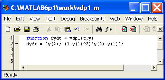
Taking the initial solution y1 = 2 and y2 = 0 in the interval [0,20], we can solve the system using the following MATLAB syntax:
>> [t, y] = ode45(@vdp1,[0 20],[2; 0])
t =
0
0.0000
0.0001
0.0001
0.0001
0.0002
0.0004
0.0005
0.0006
0.0012
.
.
19.9559
19.9780
20.0000
y =
2.0000 0
2.0000 - 0.0001
2.0000 - 0.0001
2.0000 - 0.0002
2.0000 - 0.0002
2.0000 - 0.0005
.
.
1.8729 1.0366
1.9358 0.7357
1.9787 0.4746
2.0046 0.2562
2.0096 0.1969
2.0133 0.1413
2.0158 0.0892
2.0172 0.0404
We can graph the solutions using the following syntax (see Figure 7-53):
>> plot (t, y(:,1),'-', t, y(:,2),'-')
>> xlabel ('time t')
>> ylabel('solution y')
>> legend ('y_1', 'y_2')

To solve the general system with the parameter μ, we define the system in the M-file shown in Figure 7-54.

Now we can graph the first solution y1 = 2 and y2= 0 corresponding to μ = 1000 in the interval [0,1500] using the following syntax (see Figure 7-55):
>> [t, y] = ode15s(@vdp2,[0 1500],[2; 0],[],1000);
>> xlabel ('time t')
>> ylabel ('solution y_1')

To graph the first solution y1 = 2 and y2 = 0 for another value of the parameter, for example μ= 100, in the interval [0,1500], we use the following syntax (see Figure 7-56):
>> [t, y] = ode15s(@vdp2,[0 1500],[2; 0],[],100);
>> plot (t, y(:,1),'-');

EXERCISE 7-11
The Fibonacci sequence {an} is defined by the recurrence law a1 = 1, a2 = 1, an+1 =an-1 + an. Represent this sequence by a recursive function and calculate a2, a5 and a20.
To generate terms of the Fibonacci sequence we define a recursive function in the M-file fibo.m shown in Figure 7-57.

Terms 2, 5 and 20 of the sequence are now calculated using the syntax:
>> [fibo(2), fibo(5), fibo(20)]
ans =
2 8 10946
EXERCISE 7-12
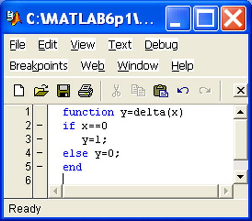
Define the Kronecker delta, which equals 1 if x = 0 and 0 otherwise. Define the modified Kronecker delta function, which is 0 if x = 0, 1 if x> 0 and -1 if x <0 and graph it. Lastly, define the piecewise function that is equal to 0 if x ≤ -3, x3 if -3 <x <-2, x2 if -2≤x≤2, x if 2<x<3 and 0 if 3≤x, and graph it.
The Kronecker delta delta(x) is defined in the M-file delta.m shown in Figure 7-58. The modified Kronecker delta delta1(x) is defined in the M-file delta1.m shown in Figure 7-59. To define the third function piece1(x) of the exercise, we create the M-file piece1.m shown in Figure 7-60.


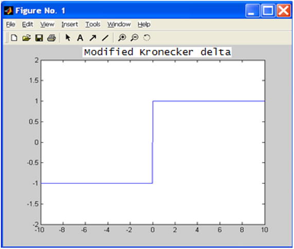
To graphically represent the modified Kronecker delta on the domain [-10, 10] (and with codomain [-2, 2]) we use the following syntax (see Figure 7-61):
>> fplot ('delta1 (x)', [- 10 10 – 2-2])
>> title 'Modified Kronecker Delta'
To graphically represent the piecewise function on the interval [- 5,5] we use the following syntax (see Figure 7-62):
>> fplot ('piece1 (x)', [- 5 5]);
>> title 'Piecewise function'

EXERCISE 7-13
Define a function descriptive(v) which returns the variance and coefficient of variation of the elements of a given vector v. As an application, find the variance and coefficient of variation of the set of numbers 1, 5, 6, 7 and 9.
Figure 7-63 shows the M-file which defines the function descriptive.

To find the variance and coefficient of variation of the given set of numbers, we use the following syntax:
>> [variance, cv] = descriptive([1 5 6 7 9])
variance =
7.0400
cv =
0.4738