
Chapter 4: Skull stripping and tumor detection using 3D U-Net
Rahul Gupta; Isha Sharma; Vijay Kumar National Institute of Technology, Hamirpur, Himachal Pradesh, India
Abstract
Skull stripping from magnetic resonance imaging (MRI) is an important field of research. Its applications and requirements in the field of medical image processing have led to a need for more research in this area, and advancements in the field have resulted in the generation of many different techniques. The model demonstrated here is based on the 3D U-Net architecture, consisting of a layered approach to segment the brain, for extraction of lower-grade gliomas from the stripped tissues. This method is capable of performing automatic skull stripping and extracting the lower-grade gliomas from an MRI dataset of the human brain. When trained appropriately this model has shown effective results via the Dice coefficient and IoU metrics, and has outperformed other existing methods. This model can be useful in estimating tumor stages because of its well-defined architecture.
Keywords
Skull stripping; Magnetic resonance imaging; Neural network; Tumor extraction; U-Net
1: Introduction
Digital image processing has been adeptly applied in medical science, increasing efficiency in the study of anatomical structure, diagnosis, surgical planning, treatment planning, research, computer integrated surgery, and many other areas. The emerging field of image processing and artificial intelligence has gained much recent attention in medical research and applications. Among all of the techniques used, MRI (magnetic resonance imaging) stands out. This technology makes use of a strong magnetic field and radio waves in order to obtain detailed images of various body organs and tissues (Rutegard et al., 2017; Smith-Bindman et al., 2012). It has high anatomical resolution and hence provides more detailed information on the anatomical structure. This is considered to be a crucial field of research, as it is necessary to reduce the need for human intervention in the preliminary step of image processing, i.e., skull stripping, or brain extraction, in which nonbrain tissues are separated from brain tissues, in order to decrease the variance and delay due to the time-consuming process of manual processing, which obstructs analysis and large-scale diagnosis and treatment. MRI is usually preferred over other techniques, as it can create efficient contrast in both the interior and exterior brain tissues, and thus it enhances the automated skull stripping process.
Medical image processing and research is a critical part of study and prognosis using magnetic resonance imaging (MRI). It is used in the study of the brain’s anatomical structure, in which image segmentation has become a vital part of neurosurgical medical research, as a highly weighted step in the process of extracting features from the image. It is easier to perform analysis of skull-stripped images; therefore an accurate and unbiased skull segmentation method has become a much-valued technique. The tissues of the brain have various important features that are used in brain segmentation. However, detecting the border of the brain can become challenging due to low contrast and artifacts, and the segmentation can easily be corrupted due to noise, bias-field effects, or partial volume effects, possibly resulting in misleading outputs that can lead to faulty observations and diagnosis. This challenge becomes more severe in the case of deformities in brain tissues, sometimes due to the presence of diseases such as tumors, Alzheimer’s disease, etc. As a result, this step is considered to be one of the challenging tasks in image processing.
Various approaches have been developed for brain tissue extraction purposes, but no one method is suitable for all types of images. There are several classical approaches that, according to Liu et al. (2014), can be categorized as region-based, boundary-based, atlas-based, and hybrid-based approaches. Also, there are many approaches based on neural networks or deep learning (Lin et al., 2016), which can easily handle bulky datasets and can justifiably derive useful information from them.
Automatic brain tumor detection is another challenging step, due to the variability of shapes and sizes, variable positions, and intensities (Rehman et al., 2020). Brain tumors are of two main types, primary and secondary, where primary tumors are noncancerous while secondary are cancerous. Due to the complexity of this task, various techniques have been developed in the past making use of the different existing imaging techniques, such as CT, PET, MRI, and multimodal imaging techniques. These provide information by using the various tissue features present in the brain. In our work we have specifically focused on the MRI imaging technique, for which there have been various methods developed for tumor detection, including thresholding methods (Singh and Magudeeswaran, 2017), region growing methods (Deng et al., 2010), edge-based methods (Aslam et al., 2015), fuzzy clustering techniques, morphological-based methods, atlas-based methods, and neural network-based methods. Apart from all the previous methods, there are still many challenges in tumor detection techniques, due to artifacts and noise interruptions. It is crucial to be able to detect tumors accurately, as the entire process of diagnosis and treatment can collapse with inefficient automatic skull stripping and tumor detection techniques. In our methodology, an effective approach has been demonstrated that can efficiently minimize these challenges by implementing a 3D U-Net approach for performing neural-based automatic skull stripping, along with supporting detection of the presence of lower-grade gliomas from the MRI dataset.
1.1: Previous work
The segmentation of brain tissues is an initial but critical step in the field of medical image processing for accurate diagnosis and surgery estimations. There are numerous generally available datasets that can be used in different skull-stripping algorithms, such as the Alzheimer’s Disease Neuroimaging Initiative (ADNI) dataset (Jack et al., 2008), which has been developed in many steps. Some of the major datasets available are: (1) ADNI1 (2004–2009), ADNI2 (2010–2016), and ADNI3; (2) Open Access Series of Imaging Studies (OASIS) dataset (Marcus et al., 2007); (3) LPBA40, which shows digital brain atlases (Shattuck et al., 2008); (4) Internet Brain Segmentation Repository (IBSR) (IBSR, 2020), which shows manually delineated results with MRI data; (5) National Alliance for Medical Image Computing (NAMIC), which consists of T2W images with skull-stripped data; and (6) Neurofeedback Skull-stripped (NFBS) database (NFBS, 2020), which is publicly available having a total of 125 MRI images with 48:77 skull-stripped datasets for men and women, respectively.
There are basically three types of MRI brain images: T1-weighted, T2-weighted, and PD-weighted images, which focus on different contrast characteristics of brain tissues (Akkus et al., 2017). Various steps are required before images of the brain can be processed, among which is segmentation, considered to be a crucial stage in image processing, as previously mentioned. A great deal of work has been proposed in this field of segmentation, which can typically be classified into two major types of approaches: classical approaches and neural network-based approaches.
In the field of classical skull-stripping approaches, morphology-based methods have been applied (Brummer et al., 1993), wherein histogram thresholding was used prior to applying morphology filters. Atkins and Mackiewich (1998) developed a multistage model. Various methods based on histogram analysis for skull segmentation were proposed by Shan et al. (2002) and Galdames et al. (2012). Another approach, called the Brain Extraction Approach (BEA), was proposed by Somasundaram and Kalaiselvi (2010, 2011); it works by adjustment of the deformable model until the expected borders are reached. The Brain Surface Extraction (BSE) approach was proposed by Shattuck et al. (2001).
Atlas-based methods are based on prior knowledge from reference images (Cabezas et al., 2011). Leung et al. (2011) proposed a multiple atlas propagation and segmentation technique (MAPS); this method generates multiple segmentations using library templates and an algorithm called simultaneous truth and performance level estimation (STAPLE). The BEaST (brain extraction based on nonlocal segmentation technique) method was developed by Manjon et al. (2014), using a sum of squared differences in order to observe the brain mask. A new multiatlas brain segmentation (MABS) method was proposed by Del Re et al. (2016). Unlike atlas-based algorithms, MABS uses weights for the atlases according to their similarity to the target image.
Region growing methods are based on pixels merging with their neighbors according to their similarity criteria. Based on this methodology, Justice et al. (1997) have presented a 3D SRG (seeded region growing) method for brain MRI segmentation. Park and Lee (2009) have presented a 2-dimensional (2D) RG for brain T1W MRIs, where seed and nonseed regions are generated using masks developed by morphological operations; however, this approach was limited for coronal orientation of brain MRIs. This limitation was handled by Roura et al. (2014) using both axial views and low-quality brain images, with a multispectral adaptive region growing algorithm (MARGA) for skull stripping. A level set approach by Wang et al. (2010) based on local Gaussian distribution fitting energy for brain extraction in MRI has given more accurate results when used in a region-based methodological approach. A drawback faced by region-based algorithms is oversegmentation of the brain tissue, which can be handled by various other methods such as hybrid models or neural network models.
In hybrid models combinations of various methods are used, according to the pros and cons of various already-proposed methodologies and imaging techniques, in order to generate the best combination of techniques for fully automating the segmentation process with better analysis and performance. A popular combination of an atlas-based active contour skull stripping algorithm with a level setting-based algorithm was devised by Bauer et al. (2012a, 2012b). BEMA, another Brain Extraction Meta Algorithm, used a combination of quad extractors along with a registration process to generate more accurate results (Rex et al., 2004). MRI brain segmentation framework was developed in two stages. Initially, all nonbrain tissues were removed and then applied automatic gravitational search algorithm to pull out brain tissues from skull stripped images (Kumar et al., 2014).
Currently, the deep learning-based approach also makes use of numerous techniques. They are easily deployable and deep learning has proved to be an accurate and unbiased approach for extracting brain masks. In Kleesiek et al. (2016) a fully neural network-based technique for skull stripping was devised, which has shown better performance than the previous classical techniques. A deep-learning technique based on the U-Net architecture was developed to attain volumetric segmentations from a sparse annotation; a DeepMedic was trained over a smaller amount of data using BRATS 2016 and was able to show outstanding results in terms of Dice. It is sustainable for datasets that require no minimal preprocessing, like BRATS 2015 and 2016. The question as to whether a model will perform in the same manner when trained on one dataset and tested on another was analyzed. Yet another method was reported by Lu et al. (2019), in which a 3D CNN architecture of three levels was used where each level is followed by pooling process along with usage of ConvNet1 and ConvNet2 models, yielding large parameters, followed by tuning of parameters in order to maintain balance between computational time and efficiency.
Tumor detection is best when achieved in the early phases of tumor building, as it can be diagnosed and treated accordingly. In this field of research and study, MRI images have shown better outputs as compared to CT scans or ultrasound. Automated tumor detection is very challenging; better outcomes are obtained with the use of convolution neural networks. In Xu et al. (2015) the methodology made use of ImageNet for extracting features and showed 97.5% accuracy in classification and 84% accuracy in segmentation. In Pan et al. (2015) multiphase MRI images for tumor grading were analyzed and a comparative study was done between deep-learning structures and base neural networks; based on the sensitivity and specificity of the CNN, the performance of the structure was improved by 18% compared to the neural networks. In a study by Siar and Teshnehlab (2019), feature extraction along with a CNN was deployed after preprocessing of images, which showed 98.67% accuracy with the Softmax classifier, 97.34% with the radial basis function (RBF) classifier, and 94.24% with the decision tree (DT) classifier.
2: Overview of U-net architecture
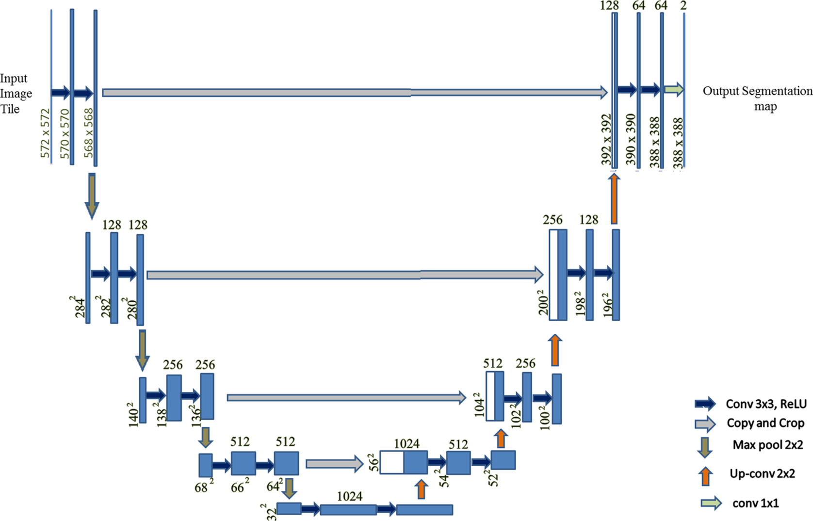
U-Net is basically a 2D convolution neural network introduced by Ronneberger et al. (2015). This network consists of normal convolutional layers and max-pooling layers followed by an equal number of up-convolutional layers. These convolutional and up-convolutional layers in the network are connected by skip connections.
2.1: 3D U-net
The 3D U-Net architecture was constructed by Cicek et al. (2016) for 3D images. In this architecture 3D kernels are used, unlike in the 2D U-Net. When tested, this architecture has been shown to train and generate prediction results for an entire voluminous image. The large memory requirement for analyzing a 3D image is a major drawback for conventional techniques, which can be easily dealt with using this architecture. The analysis path uses max pooling and performs two convolutions per max-pooling operation of kernel size 3 × 3 and with stride 1. Padding is performed on the data so that the output size comes out to be equal to the input. The U-Net architecture is especially well-suited for image segmentation. This network is a fully convolutional network, and the original reason that this architecture was developed was for use in biomedical image segmentation. The architecture is U-shaped, which is why it is called U-Net. In this architecture, the left part is called the contraction path or encoder path, whereas the right part is called the expansion path or decoder path. We can also modify the various parameters of the architecture based on the problem statement and dataset. The contraction path is used to pull out the global features. This consists of the convolution block and max pooling. The convolution block comprises the batch normalization (Ioffe and Szegedy, 2015), convolution, and an activation function called the rectified linear unit (ReLU). This architecture as shown in Fig. 1 and uses padding and maximum pooling as shown in Fig. 3.
2.1.1: Batch normalization
Normalization is used to convert various data values in common scale types of values; by using batch normalization, the neural network becomes faster and more stable.
2.1.2: Activation function
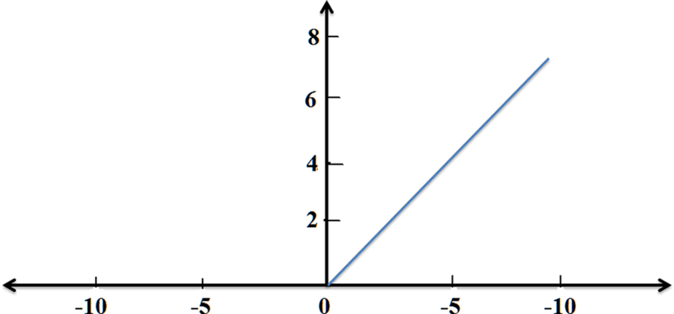
Activation functions are types of mathematical expressions used to find the output of a neural network. There are various types of activation functions, including ReLU, Leaky ReLU, Sigmoid, and so on. ReLU is one of the linear functions that gives a positive output for positive input values, else zero. This activation function is used to reduce the vanishing gradient problem, and it is used in our model also (Fig. 2).
2.1.3: Pooling
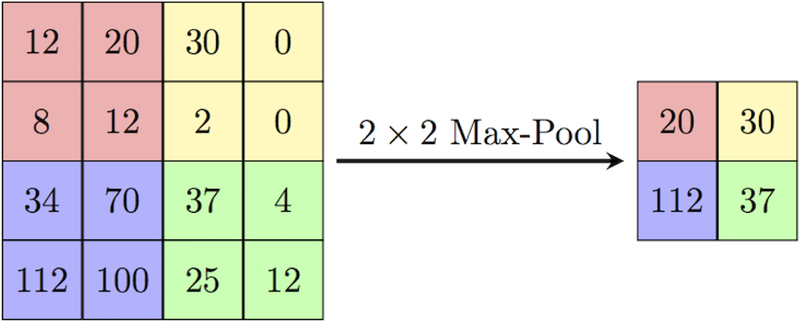
The main idea for the use of pooling is to reduce the dimension of the matrix and accept some features based on some assumptions, similar to a filter applied to the feature map. Various pooling techniques are used, such as max pooling, min pooling, mean pooling, and so on. In this U-Net architecture, max pooling is used, of size 2 × 2 pixels. This 2 × 2 size of the pooling matrix is placed on the pixels of the image and the max pixel is pulled out from that image in 2 × 2 matrixes, as shown in Fig. 3.
2.1.4: Padding
Padding can be defined as “a measure of pixels to be added to an image when it is being prepared by the kernel of a CNN.” For this U-Net architecture, padding is defined as “same”: i.e., the output image is to have the same dimensions as the input image.
2.1.5: Optimizer
Optimizers perform the adjustment of the learning rate for individual parameters. There are various algorithms for optimizing stochastic gradient descent (SGD) in neural networks, such as Momentum, Adagrad, Adadelta, RMSprop, and Adam. Adagrad is the foremost optimizer, which optimizes the image on a greater level by adding up the gradient history. Hence this makes it suitable for use with small datasets. RMSprop scales its learning rate by finding the mean of the recent gradients of the parameters. Adam is one of the most recently introduced optimizers; it uses first- and second-order momentum to scale the learning rate for each parameter.
3: Materials and methods
3.1: Dataset
The dataset used contains brain MR images together with manual FLAIR abnormality segmentation masks. The images were obtained from The Cancer Imaging Archive (TCIA). They correspond to 110 patients included in The Cancer Genome Atlas (TCGA) lower-grade glioma collection with at least fluid-attenuated inversion recovery (FLAIR) sequence and genomic cluster data available. This model was trained on 2828 MRIs with parameters as follows: number of epochs 50, batch size 32, and learning rate 0.0001. The performance of the 3D U-Net was evaluated on a dataset “LGG Segmentation Dataset” that is publicly available (LGG, 2019); the results were obtained by this model for 373 MRIs. Here, the input size of each scan was 256 × 256 × 3. In this dimension, 256 × 256 defines the length and width, respectively, whereas 3 defines the depth of scan, or RGB image.
3.2: Implementation
The implementation of this model was carried out as follows:
- Step 1: Image Acquisition.
Initially, images were collected from the dataset of both types of normal MRI and their respective mask images. - Step 2: Data Visualization.
After collecting the data, the MRI was visualized with the help of the collected dataset. For this, we imported the cv2 library and converted the BGR images to RGB images. - Step 3: Train and Test Dataset.
Then the dataset was split for the training and testing of the model. For the training, 2828 MRI sets were used, and for testing the model, 393 MRI sets were collected. - Step 4: Data Generation and Data Augmentation.
With this step, we generated image and mask at the same time and used the same seed for image data generation and mask generation to ensure the transformation of the images. - Step 5: Define U-Net Architecture.
In this step, the architecture of U-Net was defined with the ReLU and sigmoid activation function. Normalization, padding, and strides were also used to prepare the model. With this, the total parameters were 31,043,521 (trainable parameters are 31,037,633 and nontrainable parameters are 5888). - Step 6: Train the Model.
The model was trained with 50 epochs, batch size of 32, and learning rate of 0.0001. The Adam optimizer was also used to compile the model. From this, we obtained train and test evaluation metrics. - Step 7: Test the Model.
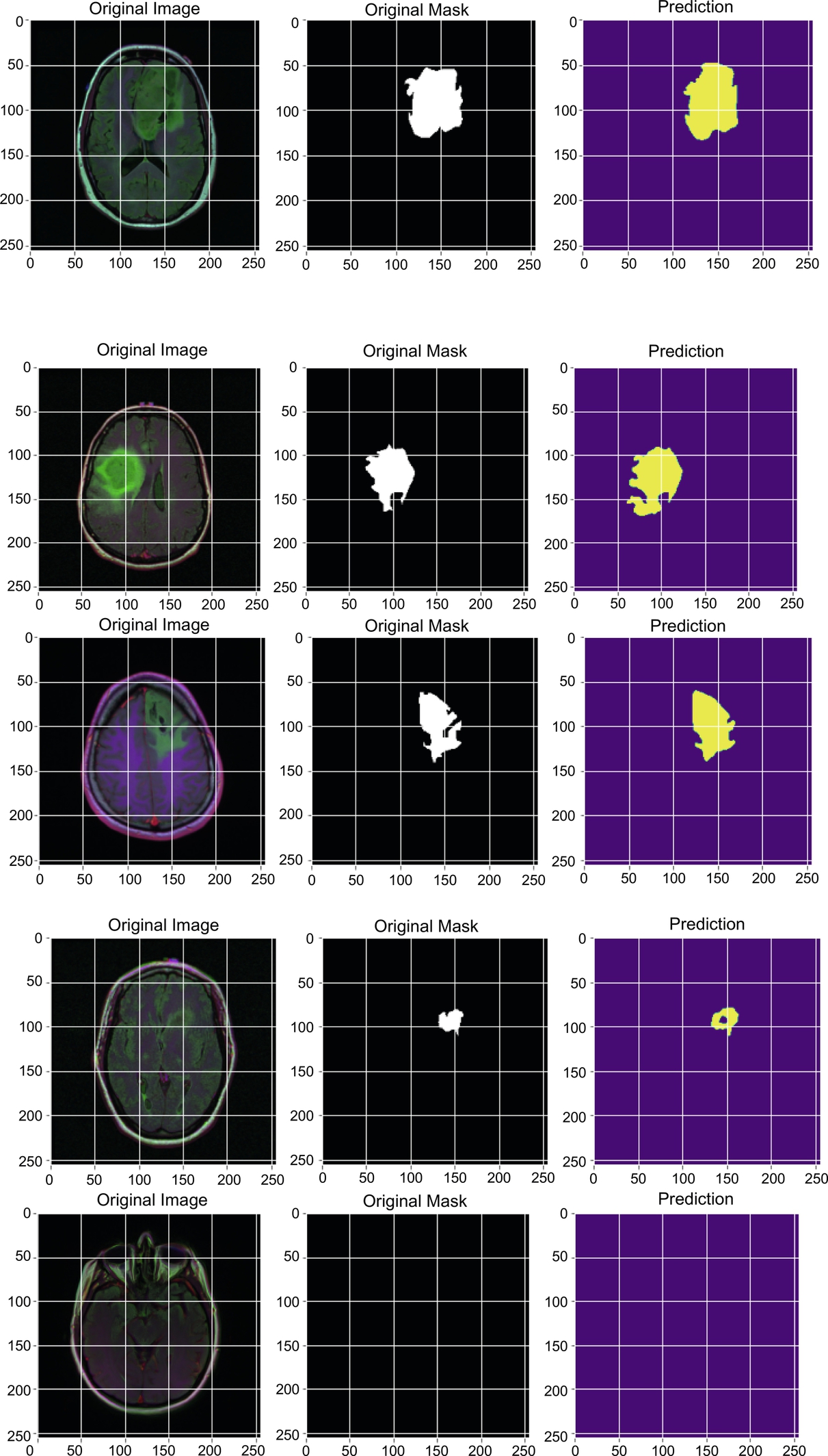
After training the model, the model was tested on 393 images and achieved better accuracy, Dice coefficient, and IoU than existing methods. Some original and predicted results as obtained by the model are shown in Fig. 5.
4: Results
4.1: Experimental result
Various implementations of skull segmentation have been done using non-deep learning methods, such as Brain Surface Extractor (BSE) and Robust Brain Extraction (ROBEX) (Iglesias et al., 2011), and also deep learning-based methods, such as Kleesiek’s method (Kleesiek et al., 2016). The BSE algorithm works by filtering the image, detecting the edges, performing a morphological operation, followed by surface cleanup to identify the brain. ROBEX is an automatic whole-brain extraction tool for T1-weighted MRI data; it aims for robust skull-stripping across datasets with no parameter settings..
4.1.1: Dice coefficient
The Dice coefficient can be defined as “the ratio of twice the intersection of the pixels of both images to the sum of all pixels of both the images.”
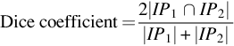
where IP1and IP2 are the image pixels of image 1 and image 2, respectively.
This can also be defined in terms of a confusion matrix:
4.1.2: Accuracy
The accuracy is the ratio of truly predicted data points out of all data points. It can also be defined as the ratio of the sum of true positive, true negative to the sum of true positive, true negative, false positive, and false negative.
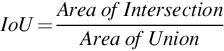
4.1.3: Intersection over Union (IoU)
Intersection over Union is the ratio of the intersection of pixels of images to the union of all the pixels of all the images. It is also called the Jaccard Index. This metric is used for image segmentation and object detection. If IoU score ≥ 0.5 then that score is considered a good score.
This model was trained on 2828 MRIs with parameters as follows: number of epochs 50, batch size 32, and learning rate 0.0001; some of the results are shown in Table 1.
Table 1
| Epochs | Accuracy | IoU | Dice Coefficient | Val_Accuracy | Val_IoU | Val_Dice coefficient |
|---|---|---|---|---|---|---|
| 1 | 0.9176 | 0.0509 | 0.0957 | 0.9890 | 0.0119 | 0.0233 |
| 5 | 0.9810 | 0.1417 | 0.2439 | 0.9886 | 0.1017 | 0.1818 |
| 10 | 0.9956 | 0.4474 | 0.6104 | 0.9958 | 0.4697 | 0.6331 |
| 15 | 0.9960 | 0.5726 | 0.7205 | 0.9946 | 0.3850 | 0.5497 |
| 20 | 0.9969 | 0.6941 | 0.8155 | 0.9972 | 0.7014 | 0.8128 |
| 25 | 0.9972 | 0.7296 | 0.8393 | 0.9970 | 0.7118 | 0.8294 |
| 30 | 0.9973 | 0.7421 | 0.8446 | 0.9969 | 0.7079 | 0.8207 |
| 35 | 0.9974 | 0.7639 | 0.8625 | 0.9972 | 0.7385 | 0.8456 |
| 40 | 0.9972 | 0.7447 | 0.8482 | 0.9958 | 0.5870 | 0.7248 |
| 45 | 0.9974 | 0.7677 | 0.8652 | 0.9975 | 0.7620 | 0.8547 |
| 50 | 0.9975 | 0.7849 | 0.8753 | 0.9976 | 0.8007 | 0.8882 |
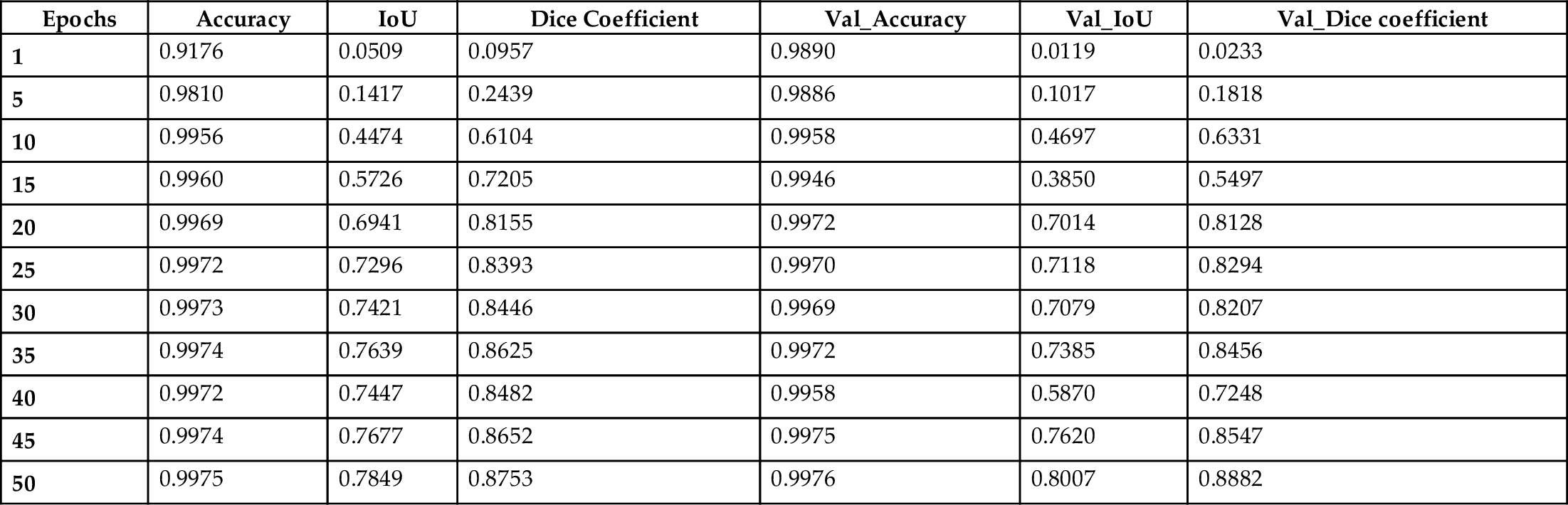
The results obtained by this model for the 373 MRIs tested using the U-Net architecture are depicted in Table 2.
4.2: Quantitative result
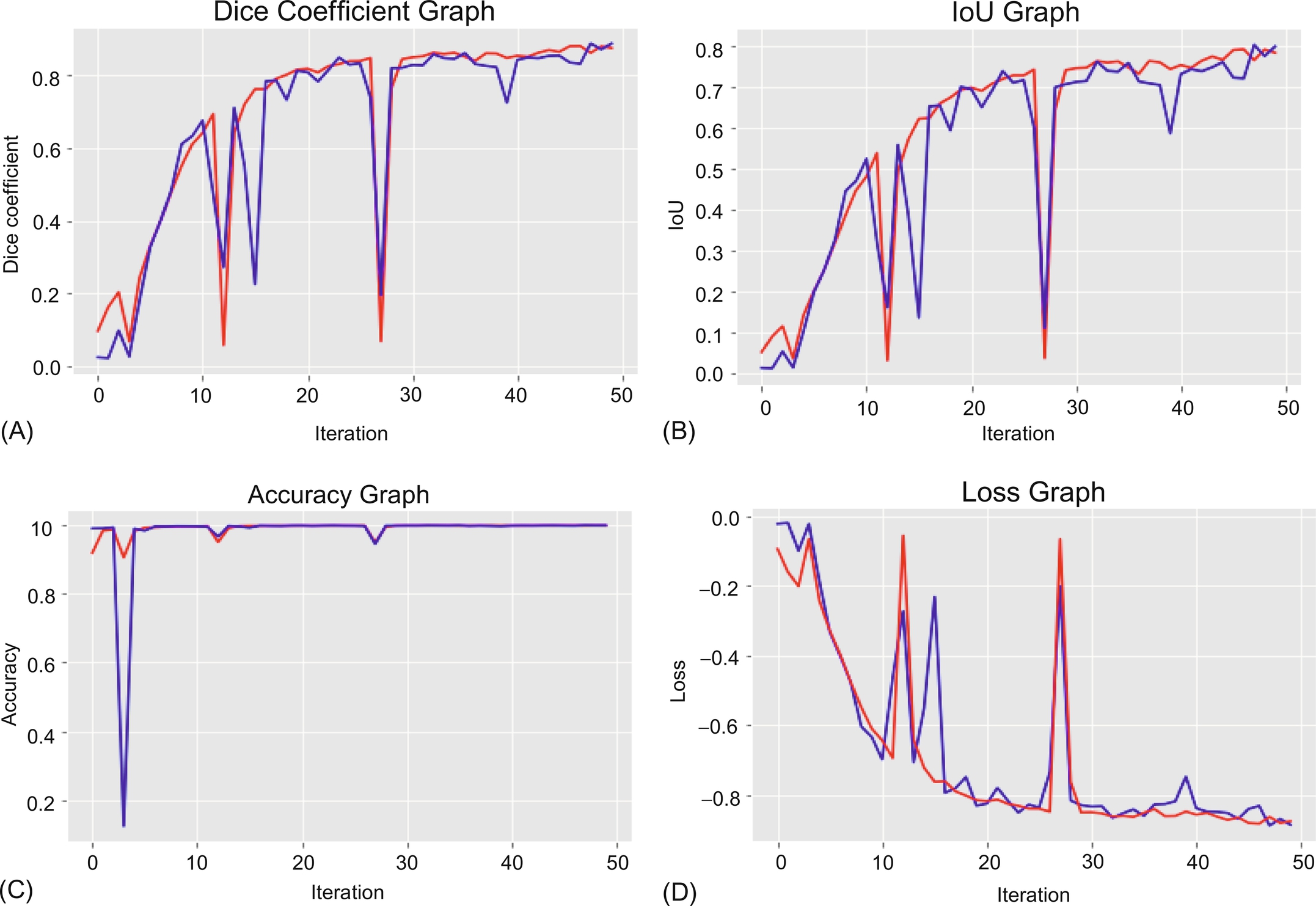
Using the Table 1 data, we can summarize in graphs, as shown in Fig. 4. Both types of data are plotted on the graph: i.e., training data is shown in red and test data is shown in blue. A graph of the entire metrics as well as a loss graph are also plotted.
4.3: Qualitative result
The model was tested on 373 MRIs with an accuracy of 0.9978. We can see the results of the images with their respective masks which were tested on the proposed model and lower-grade gliomas, using shape features which were automatically extracted by the proposed model as shown in Fig. 5.
5: Conclusion
We have implemented a 3D U-Net to segment the brain and for extraction of lower-grade gliomas from the stripped tissues. This method is capable of performing automatic skull stripping and extraction of lower-grade gliomas from the MRI dataset of the human brain that was used. When trained appropriately, this model has shown effective results according to the Dice coefficient, IoU metrics, etc., as has been demonstrated. Also, this model can be beneficial in making clear estimations of tumor stages because of the model’s well-defined architecture. We believe that the implemented technique will be useful for very large-scale case studies and treatment. In future, this approach can be modified for detection of other types of brain tumors by analysis of other features without being affected by issues of inhomogeneity.