
Chapter 12: An entropy-based hybrid feature selection approach for medical datasets
Rakesh Raja; Bikash Kanti Sarkar Department of Computer Science and Engineering, Birla Institute of Technology, Mesra, Ranchi, India
Abstract
Feature selection is an important step of data mining. The literature on feature selection techniques is very vast encompassing the applications of machine learning and pattern recognition. The techniques show that more information is not always good in machine learning applications. The ultimate goal of any feature selection method is to remove irrelevant or redundant features/attributes of datasets in order to reduce computation time and storage space, and to improve prediction performance of the learning algorithms. More generally, a feature selection algorithm is selected based on the following considerations—simplicity, stability, number of reduced features, classification accuracy, storage, and computational requirements.
Importantly, medical datasets often possess redundant features that increase learning time of disease prediction model and also degrade its performance. Plenty of feature selection methods are available in literature to improve prediction accuracy of learning models while reducing feature space dimensionality, but most of them are not stable and they lack to select the more accurate attributes in linear time.
In this study, a stable linear-time entropy-based ensembled feature selection approach is introduced, mainly focusing on medical datasets of several sizes. The suggested approach is validated using three state-of-the-art classifiers, namely C4.5, naïve Bayes, and JRIP over 14 benchmark medical datasets (drawn from UCI machine learning repository). The empirical results achieved from the datasets demonstrate that the proposed ensemble model outperforms the selected learners.
Keywords
Feature selection; Linear time, disease prediction; Accuracy
1: Introduction
In recent years, the rapid adoption of computerized Disease Decision Support Systems (DDSS) has been shown to be a promising avenue for improving clinical research (Chen and Tan, 2012; Garg et al., 2005; Kensaku et al., 2005; Moja et al., 2014; Narasingarao et al., 2009; Syeda-Mahmood, 2015; Thirugnanam et al., 2012; Wagholikar et al., 2012; Ye et al., 2002; Srimani and Koti, 2014; Gambhir et al., 2016; Subbulakshmi and Deepa, 2016; Bhardwaj and Tiwari, 2015; Sartakhti et al., 2012; Li and Fu, 2014; Fana et al., 2011; McSherry, 2011; Marling et al., 2014; Prasad et al., 2016; Singh and Pandey, 2014; Downs et al., 1996; Kawamoto et al., 2005; Sampat et al., 2005; Lisboa and Taktak, 2006). The reason for constructing DDSSs is that manual detection of diseases is prohibitively expensive, time consuming, and prone to error. However, there exist various challenges and practical limitations associated with clinical data. One big issue is to operate redundant and noisy features, many of which are correlated and/or of no significant diagnostic value. The redundant (and noisy) features unnecessarily increase the learning time of DDSS, and sometimes degrade the performance of the system. Feature-selection is the only solution of this issue.
1.1: Deficiencies of the existing models
To improve prediction accuracy of learning models by reducing feature space dimensionality, a significant number of feature-selection methods have been proposed over the years, using various schemes like probability distribution, entropy, correlation, etc. (Abdullah et al., 2014; Bhattacharyya and Kalita, 2013; Hoque et al., 2014; Swiniarski and Skowron, 2003; Breiman, 1996; Schapire, 1999). In recent years, feature selection methods are being greatly used to reduce dimensionality of data for big data analytics (Fernández et al., 2017; Kashyap et al., 2015). For comprehensive review on feature selection, one may refer the recent study (Li et al., 2017). In this chapter, it is stated that some hot topics for feature selections, e.g., stable feature selection, multiview feature selection, and multilevel feature selection have been emerged.
Although many works have been reported in the literature, there is still scope for improvement. For example, most of them are not stable and lack to select the more accurate attributes from dataset in linear time.
Contribution: Addressing the issues of the existing models, a stable linear time entropy-based feature-selection approach is introduced in the present chapter, mainly focusing on medical datasets of different sizes. In particular, stability is the sensitivity of the chosen feature set to variations in supplied training dataset. More specifically, how much the model is sensitive to the small changes in the dataset? Undoubtedly, such model is important, especially in medical datasets.
1.2: Chapter organization
The rest of the chapter is organized as follows. In Section 2, a brief discussion is given on feature selection, whereas the methodology proposed in this research is explained in Section 3. The experimental results are presented in Section 4, whereas the obtained results are analyzed in Section 5. Conclusions and future scopes are presented in Section 6.
2: Background of the present research
2.1: Feature selection (FS)
The term feature selection refers to the process of selecting the optimal features (i.e., only the most relevant features). In other words, it aims to reduce the inputs for processing and analysis. Owing to several dependent features in datasets (especially in medical datasets), feature engineering needs to be employed to select the most important ones that are likely to have a greater impact on our final model. The prime goal of any feature selection approach is to select a subset of features from the input which can efficiently describe the input data while reducing noisy or irrelevant features (accordingly reducing training time of learner and avoiding the case of overfitting model) and aims at good prediction results (Guyon and Elisseeff, 2003). In particular, when two features are perfectly correlated, only one feature is sufficient to describe the data. The dependent features provide no extra information about the classes, and thus serve as noise for the predictor. This means that the total information content can be obtained from fewer unique features which contain maximum discrimination information about the classes. Hence by eliminating the dependent variables, the amount of data can be reduced which can lead to improvement in the classification performance. More specifically, irrelevant and redundant attributes which do not have significance in classification task are reduced from the dataset.
In practice, two approaches are employed to reduce dimensionality of datasets. These are, namely feature selection and feature-extraction. Feature selection (FS) involves selection (but not transformation) of features using certain optimization function, whereas feature extraction allows transformation of features. More specifically, feature selection finds a subset of optimal features, whereas feature extraction creates a subset of new features by combinations of the existing features.
Obviously, feature selection is one of the preprocessing techniques in data mining. Several methods exist in literature for feature selection. In practice, the methods are grouped into three categories, namely filter, wrapper, and hybrid model (Witten Ian and Eibe, 2005). These are briefly explained.
- • Filter method: The filter method relies on general characteristic of data to evaluate and select feature subsets without involving any mining algorithm. These are typically faster and give an average accuracy for all the classifiers. This method mainly focuses on elimination of feature (columns) with more missing values, elimination of features consisting of difference between maximum and minimum values of attribute with very less, and elimination of features with high correlation among themselves. Filters are usually less computationally intensive. Examples include information gain, chi-square test, fisher score, correlation coefficient, and variance threshold.
- • The wrapper model requires one predetermined mining algorithm and uses its performance as the evaluation criteria. The wrapper methods can result high classification accuracy than filter methods for particular classifiers but they are less cost effective. Thus, the wrapper methods primarily focuses on the following point.
- • Selection of a set of features that result in comparatively high classification accuracy and low error rate
In short, the wrapper methods attempt to find a subset of features and train a learner to get its performance. So, it is comparatively expensive. The wrapper methods usually work on recursive approach that may be of two types—forward selection and backward selection. In forward selection, features are included into a set of selected features (starting with a null set) one by one to improve the performance of the learners until no improvement is observed. This results in a set of the best features. On the other hand, the backward strategy attempts to discard the feature set (starting with the complete/original set of features) one by one to improve the performance of the learners. The process stops when no improvement of the learners is found. Here, the worst features are discarded from the original set. The wrapper models are comparatively computationally intensive, but it is true that selection of optimal feature subset is an NP-hard problem (Liu and Yu, 2005), which is not solvable in polynomial time. For tackling NP-hard problems, the most commonly used random search method—Genetic algorithm (GA)—is treated as the best solution (Goldberg, 1989). In a survey paper on feature selection (Chandrashekar and Sahin, 2014), Chandrashekar and Sahin have shown that GA may be treated as the best strategy for designing wrapper model to result in the best-performing feature set for that particular type of model or typical problem. - • Embedded models: These models use the algorithms that adopt built-in feature selection methods. For instance, principal component analysis (PCA) and random forest have their own feature selection methods. These approaches tend to be between filters and wrappers in terms of computational complexity.
Lastly, we may design some hybrid approaches (a specific case of ensemble approach) that are usually the combination of filter and/or wrapper models. No matter, feature-selection improves the performance of classifiers and it reduces the learning time, as there is less number of features (as compared to the original set).
Thus, any feature selection process usually consists of the following steps.
- (i) Identification of a candidate subset of attributes from an original set of features using some searching techniques.
- (ii) Evaluation of the subset to determine the relevancy toward the classification task using measures such as distance, dependency, information, consistency, and classifier’s error rate.
- (iii) Setting termination condition to decide the relevant subset or optimal feature subset.
- (iv) Validation of the selected feature subset.
In the present research, feature selection technique (under filter category) is used to reduce the dimensionality of dataset.
3: Methodology
3.1: The entropy based feature selection approach
In 2000, Hall reported that the attributes having strong correlation cannot be the part of feature subset (Hall, 2000). It was also stated in his article that if the attributes are more independent among themselves, then the more information gain they have. Hence, it is expected to give improved results over unseen data. Interestingly, the present research focuses on medical datasets. As medical datasets are more sensitive, so stable feature selection approach is more effective for such datasets. With this point in mind, a stable simple entropy-based approach is introduced here and it is described below.
For better understanding the model, a conceptual model is shown in Fig. 1.
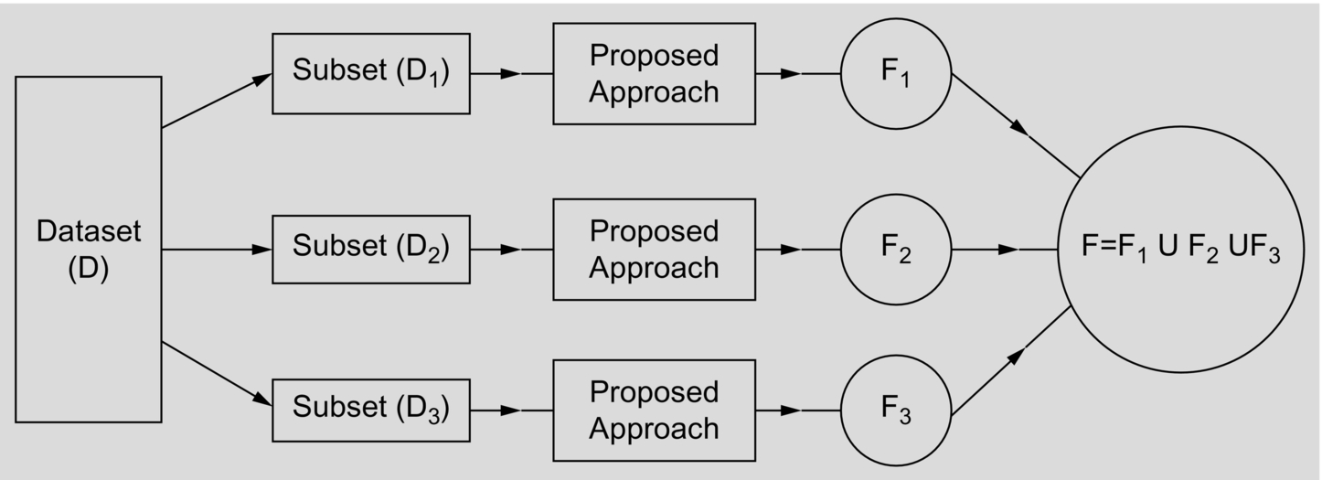
Before applying the proposed feature selection approach on any dataset (D), it is first discretized by minimum information loss (MIL) discretizer (Sarkar et al., 2011b), and each discretized dataset (D) is then split into 3 subdatasets, namely D1, D2, and D3 based on equi-class distribution data-partitioning scheme as follows. The idea on equi-class distribution is first illustrated below. For understanding the effect of equi-class distribution method, one may refer to article cited herein (Sarkar, 2016).
3.1.1: Equi-class distribution of instances
According to the concept of equi-class distribution, same percentage of examples of each class is to be included in the training set.
Illustration: Suppose 30% examples of each class from a dataset (D) are to be randomly included in a set say T. Assume that there are 3 class values (say c1, c2, and c3) and total 150 examples in D and the numbers of examples of class types: c1, c2, and c3 are respectively 33, 42, and 75. Then 10, 13, and 23 examples of class types: c1, c2, and c3 (based on the concept of ceil function, e.g., ![]() ) are included in T by random selection over D.
) are included in T by random selection over D.
3.1.2: Splitting the dataset D into subsets: D1, D2, and D3
- • D1 (1st subset): Here, 30% examples of each class are randomly drawn from D and included them in D1 but the selected instances are not removed from D.
- • D2 (2nd subset): 30% examples of each class are again selected at random from D to include them in D2 but attention is paid to include several distinct instances of D into D2.
- • D3 (3rd subset): Rest of examples of D (not in D1 and D2) are placed in D3. This is fully an independent dataset.
Suppose the dataset (D) has n attributes, say Ai, i = 1, …n. Let Fs denote a set of features and Fs = {A1, A2, …, An}.
As D is here split into 3 subsets: D1, D2, and D3, so we will get three sets of selected features, each from a distinct subset of data. Suppose these feature sets are F1, F2 and F3. Initially, Fk (k = 1, 2, 3) = Fs. Let F be the resulting feature set obtained from F1, F2 and F3.
Assume that P is a classification problem with n attributes, say Ai (i = 1, …n). Let F denote a set of features. Initially, F = Fs = {A1, A2, …, An}.
- 1. for each sub-dataset (Dk, k = 1, 2, 3) dobegin
- 2. for each attribute Ai (i = 1, .. n)dobegin
- 3. Find information-gain for Ai (i.e., Gain(S, Ai)) applying the formula:
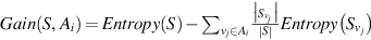 , where vj (j = 1,..k) denotes values of attribute Ai and
 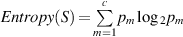 , where S represents the number of examples in P, and pm is the nonzero probability of Sm examples (out of S) belonging to class m, out of c classes.
endfor - 4. Compute r = ((max_Gain(S, Ai) − min _Gain(S, Ai))/n, (i = 1, …, n)
// (max_Gain(S, Ai) and min_Gain(S, Ai)(i = 1, …, n), are respectively the maximum and the minimum information gain among all the attributes. - 5. for each attribute Ai (i = 1, …, n)do
begin - 6. If Gain(S, Ai),(i = 1, ..n) < r, then update the feature set (Fk) as: Fk = Fk- {Ai} // discarding Aifrom F
endfor
endfor - 7. F = F1 U F2 U F3
/* F includes the common and noncommon attributes of F1, F2, and F3. As dataset corresponding to F1, F2 and F3 are balanced or close to balanced, so the chance of occurring common attributes in F1, F2 and F3 increases. */.
Note: The computed value of r = ((max_Gain(S, Ai) − min _Gain(S, Ai))/n, (i = 1, …, n), is decided as the threshold value for filtering features. The reason is that if the difference is very high for a dataset, then the dataset may have several features possessing very less contribution in building expert system, and these may be ignored from the feature set. On the other hand, if the difference is very low, then each of them plays almost equal role in designing expert system. This strategy is a kind of filtration technique for feature selection based on simple search strategy. It is explained in Appendix A.
Complexity analysis: The algorithm is very simple and straightforward. Its running time is simply O(n), where n is the number of attributes in the dataset. The approach is implemented in Java-1.4.1.
4: Experiment and experimental results
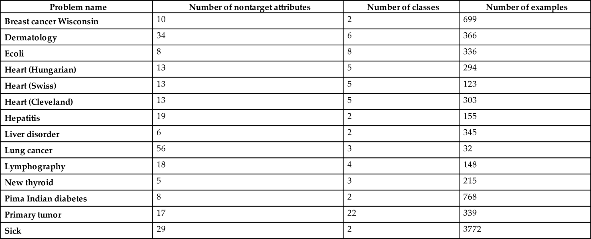
This section first describes the experiments conducted in the present research over 14 real-world benchmark medical datasets drawn from UCI data repository (Blake et al., 1999). The datasets are of different sizes, e.g., comparatively large dataset with high dimension, high-dimensional but small sample-sized data, and medium-sized dataset with less number of features. The datasets are summarized in Table 1. The obtained results are arranged in tables and the results are then analyzed.
Table 1
| Problem name | Number of nontarget attributes | Number of classes | Number of examples |
|---|---|---|---|
| Breast cancer Wisconsin | 10 | 2 | 699 |
| Dermatology | 34 | 6 | 366 |
| Ecoli | 8 | 8 | 336 |
| Heart (Hungarian) | 13 | 5 | 294 |
| Heart (Swiss) | 13 | 5 | 123 |
| Heart (Cleveland) | 13 | 5 | 303 |
| Hepatitis | 19 | 2 | 155 |
| Liver disorder | 6 | 2 | 345 |
| Lung cancer | 56 | 3 | 32 |
| Lymphography | 18 | 4 | 148 |
| New thyroid | 5 | 3 | 215 |
| Pima Indian diabetes | 8 | 2 | 768 |
| Primary tumor | 17 | 22 | 339 |
| Sick | 29 | 2 | 3772 |
4.1: Experiment using suggested feature selection approach
The implemented feature selection approach is run over 14 selected datasets. A list of selected features of the datasets is presented in Table 2. The table describes respectively the name of each dataset (denoted as DN), number of instances (NI), number of features (NF), number of selected feature (NSF), and the selected features (SF). The importance of the introduced approach is affirmed through the performance of the classifiers, viz., J48 (Java version of C4.5 (Quinlan, 1993)), naïve Bayes (Duda and Hurt, 1973) and JRIP (Java version of RIPPER (Cohen, 1995)) over the dataset (before and after selecting their features) shown in Tables 3 and 4, respectively.
Table 2
| Name of dataset (DN) | Number of instances (NI) | Number of features in the original datasets | Number of selected features | Selected features |
|---|---|---|---|---|
| Breast cancer Wisconsin | 699 | 10 | 6 | 1, 3, 4, 5, 6, 9 |
| Dermatology | 366 | 34 | 21 | 2, 3, 4, 5, 6, 7, 9,13,14,15,16, 19, 20, 21, 22, 26, 27, 28, 29, 30, 33 |
| Ecoli | 336 | 8 | 6 | 1, 2, 3, 5, 6, 7 |
| Heart (Hungarian) | 294 | 13 | 6 | 2, 3, 6, 9, 10, 11 |
| Heart (Swiss) | 123 | 13 | 3 | 9,10,11 |
| Heart (Cleveland) | 303 | 13 | 8 | 2, 3, 8, 9, 10, 11, 12, 13 |
| Hepatitis | 155 | 19 | 9 | 1, 2, 6, 11, 12, 14, 17, 18, 19 |
| Liver disorder | 345 | 6 | 2 | 3, 5 |
| Lung cancer | 32 | 56 | 17 | 1, 3, 5, 9, 13, 14, 15, 20, 21, 25 26, 38, 41, 45, 48, 50, 56 |
| Lymphography | 148 | 18 | 10 | 1, 2, 7, 8, 9, 11, 13, 15, 16, 18 |
| New-thyroid | 215 | 5 | 5 | 1, 2, 3, 4, 5 |
| Pima-Indians | 768 | 8 | 4 | 2, 6, 7, 8 |
| Primary tumor | 339 | 17 | 12 | 1, 2, 3, 4, 5, 7, 9, 10, 13, 15, 16, 17 |
| Sick | 3772 | 29 | 8 | 1, 8, 10, 14, 15, 20, 24, 29 |
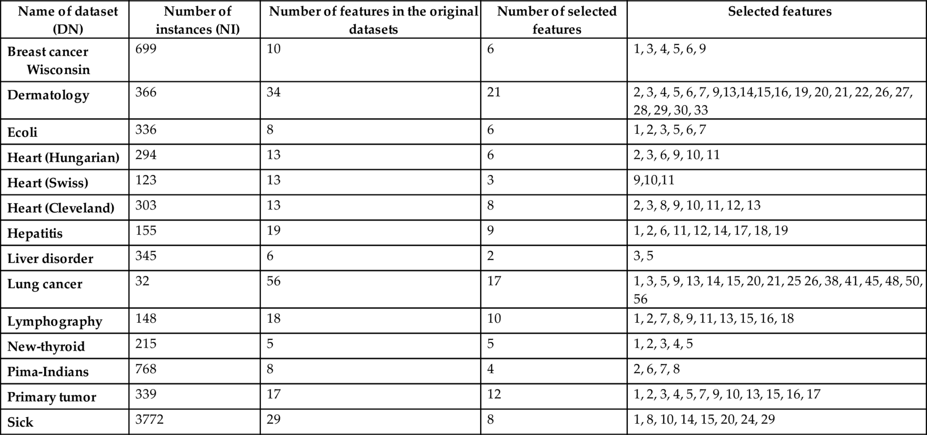
Table 3
| Problem name | Number of nontarget attributes | J48 (acc. ± s.d.) | JRIP (acc. ± s.d.) | Naïve Bayes (acc. ± s.d.) |
|---|---|---|---|---|
| Breast cancer | 10 | 73.28 ± 6.05 | 71.45 ± 6.45 | 74.70 ± 7.74 |
| Dermatology | 34 | 90.11 ± 3.34 | 86.61 ± 4.89 | 91.01 ± 2.41 |
| Ecoli | 8 | 82.13 ± 5.73 | 81.41 ± 6.30 | 84.51 ± 5.46 |
| Heart (Hungarian) | 13 | 78.22 ± 7.95 | 79.57 ± 6.64 | 80.95 ± 6.27 |
| Heart (Swiss) | 13 | 36.45 ± 13.73 | 38.08 ± 9.36 | 36.38 ± 13.13 |
| Heart (Cleveland) | 13 | 76.94 ± 6.59 | 78.95 ± 6.77 | 81.34 ± 7.20 |
| Hepatitis | 19 | 77.22 ± 9.57 | 76.13 ± 9.04 | 81.81 ± 9.70 |
| Liver disorder | 6 | 62.84 ± 7.40 | 68.57 ± 7.55 | 54.89 ± 8.83 |
| Lung cancer | 56 | 68.25 ± 21.50 | 73.92 ± 19.15 | 76.42 ± 21.12 |
| Lymphography | 18 | 74.84 ± 11.05 | 75.11 ± 11.37 | 82.13 ± 8.89 |
| New-thyroid | 5 | 93.11 ± 4.32 | 94.01 ± 4.57 | 94.16 ± 3.16 |
| Pima-Indians | 8 | 73.89 ± 5.27 | 74.18 ± 4.54 | 75.75 ± 5.32 |
| Primary tumor | 17 | 41.139 ± 6.94 | 38.74 ± 5.57 | 47.71 ± 6.46 |
| Sick | 29 | 93.13 ± 0.55 | 93.29 ± 0.68 | 92.88 ± 1.36 |
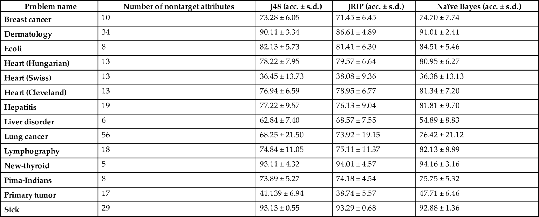
Note:acc. is simply accuracy percentage, whereas s.d. stands for standard deviation.
Table 4
| Problem name | Number of nontarget attributes after reduction | J48 (acc. ± s.d.) | JRIP (acc. ± s.d.) | Naïve Bayes (acc. ± s.d.) |
|---|---|---|---|---|
| Breast cancer | 6 (10) | 78.71 ± 1.39 | 76.97 ± 2.03 | 80.13 ± 1.23 |
| Dermatology | 21 (34) | 90.88 ± 1.20 | 88.15 ± 2.18 | 92.14 ± 1.23 |
| Ecoli | 6 (8) | 82.49 ± 2.46 | 80.91 ± 1.82 | 85.61 ± 1.19 |
| Heart (Hungarian) | 6 (13) | 78.84 ± 1.19 | 80.06 ± 1.81 | 84.07 ± 1.10 |
| Heart (Swiss) | 3 (13) | 38.26 ± 3.14 | 38.02 ± 2.39 | 38.83 ± 2.82 |
| Heart (Cleveland) | 8 (13) | 78.55 ± 2.01 | 80.15 ± 2.35 | 83.81 ± 1.48 |
| Hepatitis | 9 (19) | 80.95 ± 3.38 | 78.99 ± 3.41 | 86.45 ± 2.11 |
| Liver disorder | 2 (6) | 62.15 ± 2.72 | 69.04 ± 2.07 | 56.81 ± 2.01 |
| Lung cancer | 17 (56) | 70.74 ± 7.28 | 73.24 ± 6.12 | 79.02 ± 4.37 |
| Lymphography | 10 (18) | 74.99 ± 2.03 | 74.75 ± 3.32 | 82.94 ± 1.75 |
| New-thyroid | 5 (5) | 93.08 ± 1.09 | 93.20 ± 1.42 | 94.30 ± 0.68 |
| Pima-Indians | 4 (8) | 74.43 ± 1.88 | 74.09 ± 2.31 | 77.47 ± 1.19 |
| Primary tumor | 12 (17) | 40.81 ± 1.83 | 39.22 ± 1.92 | 47.72 ± 1.12 |
| Sick | 8 (29) | 92.89 ± 0.09 | 93.19 ± 0.04 | 93.13 ± 0.08 |
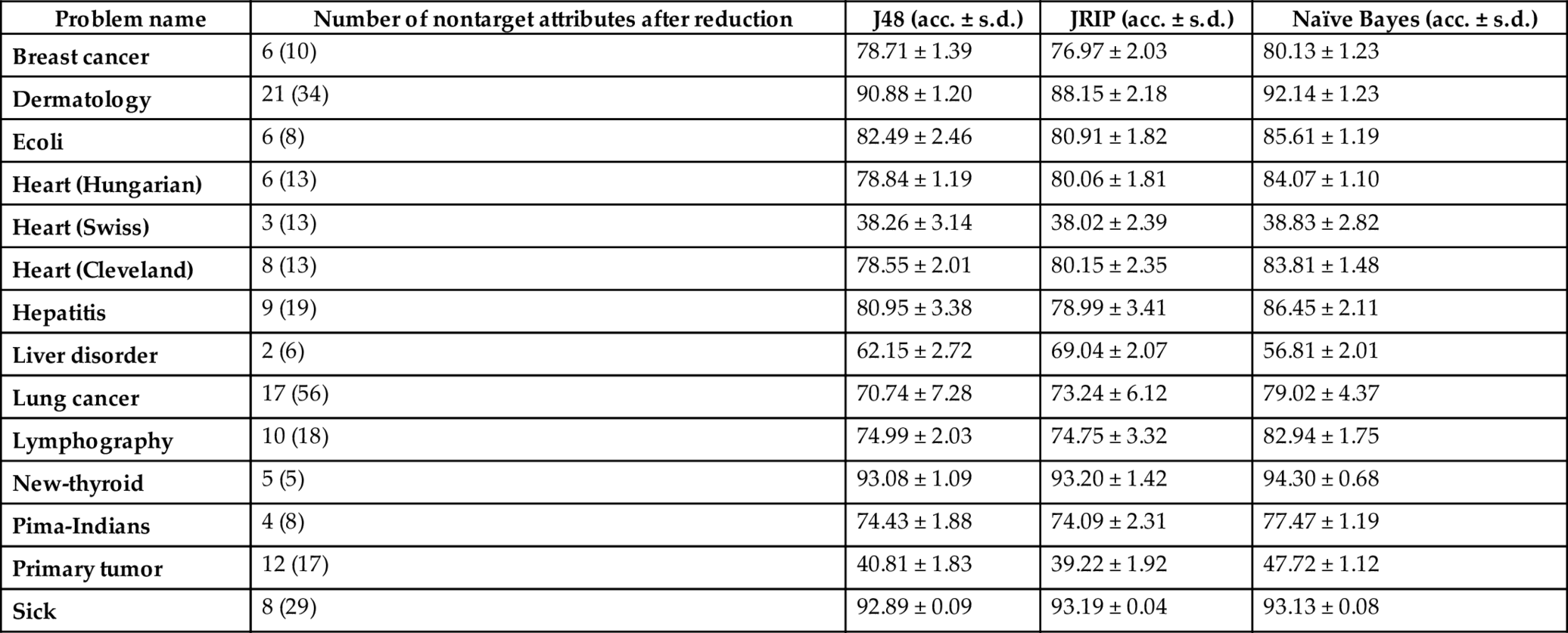
Note: Count within parenthesis placed in the second column gives the number of features in the original dataset.
In particular, naïve Bayes learner is chosen because it works better on datasets with independent features and the suggested feature selection approach focuses on identifying such features. On the other hand, JRIP is chosen, since it pays attention to select pure/correct rules. Further, the DT-based classifier C4.5 gives an average all datasets. For better estimation of the classifiers, 10-fold cross validation scheme is run 10 times in the WEKA toolbox.
Looking into Table 1, it is clear that the datasets, namely Breast cancer, Dermatology, Primary tumor, and Sick are comparatively large datasets with more features, whereas datasets, namely heart (Swiss), hepatitis, and lung cancer are the examples of high dimensional small-sized datasets. The remaining datasets (presented in Table 1) are the medium-sized datasets with less number of features.
5: Discussion
5.1: Performance analysis of the suggested feature selection approach
From the accuracy results yield by the selected learners over the datasets (displayed in Tables 3 and 4), the following points may be highlighted.
- • The accuracy (%) of the competent classifiers increases in almost all cases after removing their redundant features. In particular, the performance of naïve Bayes classifier improves significantly in almost all cases and it indicates that the introduced feature filtration method is good enough for reducing features. The reason behind the claim is that naïve Bayes classifier works better over datasets with independent features and the suggested approach aims to select such attributes. Actually, the features with very less amount of contribution (i.e., less information gain) are removed from the set when the filtration approach is applied. In other words, we may demand that the dependent features are removed from the datasets.
- • The datasets with reduced features are much reliable, since standard deviation (s.d.) of the accuracy results yielded by the classifiers are less as compared to the standard deviation of the accuracies calculated over the original ones.
Due to feature reduction, the learning time of the proposed hybrid model will be reduced to a great extent, and the size of each induced rule will be small.
6: Conclusions and future works
At the end of this study, it may be once again pointed out that the techniques of feature selection and extraction seek to compress the dataset into a lower dimensional data vector so that classification accuracy can be increased.
The literature on feature selection techniques is very vast encompassing the applications of machine learning and pattern recognition. Comparison between feature selection algorithms is appropriate using a single dataset, since each underlying algorithm behaves differently for different data. Feature selection techniques show that more information is not always good in machine learning applications.
In this paper, an entropy-based hybrid feature selection method is introduced which combines subsets of features selected over different subsets of dataset and yields an optimal subset of features. To evaluate the performance of the model, classifiers, viz., C4.5 (decision tree-based), JRIP (sequential covering), and naïve Bayes on the datasets drawn from UCI data repository are applied. The overall performance has been found to be excellent for all these datasets.
Conflict of interest
The study is not funded by any agency. It does not involve other human participants and/or animals. The author declares that there is no conflict of interests regarding the publication of this paper.
Appendix A
Classification problem: A classification problem (P) is described by a set of attributes categorized as: nontarget (i.e., feature) attribute and class (also known as target) attribute. Each problem contains only one target attribute but many feature attributes.
For better understanding the classification problem, let us consider the “golf-playing” problem. The problem takes here four feature attributes viz., Outlook, Temperature, Humidity and Windy. The target is named Playing-decision. The feature attributes are denoted as respectively A1, A2, A3 and A4, whereas C is used for the class attribute. The possible nondiscretized values of the attributes are noted below.
| Name of attribute | Values |
|---|---|
| Outlook (A1) | Sunny, overcast, rain |
| Humidity (A2) | High, normal |
| Temperature (A3) | Hot, mild, cool |
| Windy (A4) | Strong, weak |
| Playing-decision (C) | No, yes |
A nondiscretized dataset of 14 days observations for this problem is shown in Table A.1. Here, Di (i = 1, …, 14) represents day.
Table A.1
| SI. no. | Nontarget attributes (Ai, i = 1, …, 4) | Playing-decision | |||
|---|---|---|---|---|---|
| Outlook (A1) | Temperature (A2) | Humidity (A3) | Windy (A4) | ||
| D1 | Sunny | Hot | High | Strong | No |
| D2 | Sunny | Hot | High | Strong | No |
| D3 | Overcast | Hot | High | Weak | Yes |
| D4 | Rain | Mild | High | Weak | Yes |
| D5 | Rain | Cool | Normal | Weak | Yes |
| D6 | Rain | Cool | Normal | Strong | No |
| D7 | Overcast | Cool | Normal | Strong | Yes |
| D8 | Sunny | Mild | High | Weak | No |
| D9 | Sunny | Cool | Normal | Weak | Yes |
| D10 | Rain | Mild | Normal | Weak | Yes |
| D11 | Sunny | Mild | Normal | Strong | Yes |
| Dl2 | Overcast | Mild | High | Strong | Yes |
| Dl3 | Overcast | Hot | Normal | Weak | Yes |
| D14 | Rain | Mild | High | Strong | No |
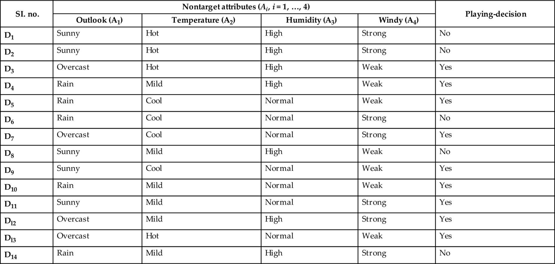
![]() , where S represents the number of currently considered learning examples and pi is the nonzero probability of the examples (say Si in S) belonging to class i, out of c classes. Here, number of nontarget attributes (features) is 4 and the number of classes is 2.
, where S represents the number of currently considered learning examples and pi is the nonzero probability of the examples (say Si in S) belonging to class i, out of c classes. Here, number of nontarget attributes (features) is 4 and the number of classes is 2.
A.1: Explanation on entropy-based feature extraction approach
The initial entropy (i.e., impurity) in the training set was:
Now,
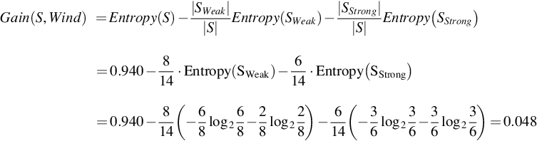
Likewise,
Gain(S, Outlook) = 0.246 is the maximum information gain, whereas Gain(S, Temperature) = 0.029 is the minimum information gain.
Thus, r = (0.246–0.029)/n = (0.246–0.029)/4 = 0.05425, since n (number of attributes) = 4. Here, each of the two attributes—Outlook and Humidity—has gain-information greater than or equal to r = 0.05425. Now, based on the suggested threshold criteria, two attributes, namely, Temperature and Windy, may be removed from the dataset, since each of the attributes—Temperature and Windy—carries very less information and the gain-information is less than the value of r.